flowchart TD
    A[Global Frequency Control] --> B[Twenty Harmonic Oscillators]
    B --> C[Individual Envelope Generation]
    C --> D[Audio Signal Collection]
    D --> E[Mixed Output]
    F[Global Time Scaling] --> C

    style A fill:#e1f5fe
    style E fill:#f3e5f5
    style C fill:#fff3e0
4 Sound Synthesis
Sound synthesis is the art and science of producing sound, whether by transforming existing recordings or by generating new audio signals electronically or mechanically. It can be grounded in mathematics, physics, or even biology, and it emerges at the intersection of creative expression and technical knowledge. As both a musical and computational process, synthesis enables the shaping of sound with precision and imagination, allowing for the creation of sonic textures that range from the familiar to the entirely new.
At its core, synthesis is a process of construction—a method for bringing elements together into a cohesive whole. This notion of “making” is essential, as it signals not just assembly, but intention. Synthesis is inherently creative. While the tools and technologies involved—oscillators, filters, software environments like Pd—are increasingly accessible and powerful, they remain just that: tools. It is the skill, intuition, and aesthetic sensibility of the artist or programmer that gives them meaning.
Modern tools have made sound synthesis more available than ever. From high-fidelity sample libraries to algorithmic engines capable of real-time manipulation, the technological barrier has lowered dramatically. But while the means have changed, the importance of the human element remains. Without creative intention, sound synthesis risks becoming a purely mechanical operation.
It is a common misconception to associate synthesis solely with complex or futuristic electronic timbres. In fact, synthesized sound spans a vast range—from simple sine waves to layered, expressive textures. The process itself is plural: it includes subtractive, additive, granular, physical modeling, and many other techniques. Each offers a different lens on how sound can be built and manipulated.
Interestingly, the term “synthesis” has roots that extend beyond audio. It also refers to the creation of new compounds in chemistry or the combining of ideas into a theory. In sound, as in those other domains, synthesis implies thoughtful construction—a deliberate act of shaping something new from constituent parts. Throughout this chapter, we will return often to the idea of synthesis not just as a technique, but as a mode of inquiry and expression. It invites experimentation, demands understanding, and rewards careful listening.
Oscillatory motion will be analyzed in detail—not only in terms of technical implementation but also through its creative and conceptual applications. Using example Pd patches provided, we will explore how oscillation becomes an expressive tool in interactive works and live sound experiments. This approach will form the core of the module’s practical component, where students are encouraged to adapt the exercises to their own interests: whether by replicating existing works, developing new compositions, or analyzing the results of comparative experiments between different oscillators and their spectral behaviors.
4.1 Between Technique and Aesthetics
This chapter begins with the idea of delving deeper into oscillatory movements from both a technical and aesthetic perspective. Building upon tools introduced in previous chapters we will work with oscillators and explore their many applications. Drawing on the text The Poetics of Signal Processing (Sterne and Rodgers 2011), we will approach signal processing not merely as a set of mathematical operations, but as a form of artistic expression. We will explore what could be described as the “rawness” of analog oscillators—that tangible, organic quality inherent in their operation. We will examine how this rawness both contrasts with and complements the digital techniques we’ve developed so far. The use of oscillators in their various forms will serve as a starting point for a series of hands-on exercises, where theory and practice are deeply intertwined.
Through this combination of theory, practice, and critical reflection on signal processing, the module aims to open up new sonic possibilities. The references provided are intended not only to contextualize student work, but also to inspire expanded thinking about how these principles might inform personal projects. This practical and flexible framework is reflected in the module’s initial activity on oscillatory movement. Readers will have the freedom to choose their working environment and the context in which they wish to develop their experiments. Oscillator implementation can be approached from multiple angles: waveform manipulation, waveshaper design, or even the creation of interactive sound pieces. In this way, the module not only deepens our understanding of the technical aspects of signal processing, but also invites critical reflection on the role of these technologies in shaping meaning and sonic aesthetics. Special emphasis is placed on the oscillator’s capacity to act as a driver of creativity and expression.
4.1.1 Poetics of Signal Processing
One of the most important aspects of this chapter is the idea of “poetics” in signal processing. This concept is not just about the technical aspects of sound manipulation, but also about the cultural and artistic implications of these processes. The term “poetics” suggests a deeper engagement with the materiality of sound and its representation in various contexts. I’m going to talk a bit about my reflections and observations on the text Poetics of Signal Processing (Sterne and Rodgers 2011). First, I want to mention the authors, who I find very interesting. The first is Jonathan Sterne, a professor and director of the Culture and Technology program at McGill University in Canada. His work focuses on the cultural dimension of communication technologies, and he specializes in the history and theory of sound in the modern Western world. Then we have another author, a sound artist and musician named Tara Rodgers. She’s an electronic music composer, programmer, and historian of electronic music. She holds a PhD in Communication and has worked in the field of Women’s Studies. She created the platform Pink Noises, which is worth checking out—especially because it gathers a series of interviews with improvisers, composers, and instrument builders. There’s a cross-section of gender, sexuality, feminism, music, sound studies, theater, performance, and performative arts in general.
Let’s get into some comments on specific sections of the article. The first is “The Sonic Turn,” which describes the emergence of a new culture of listening beginning in the second half of the 20th century. This is discussed through the work of authors like Cox and Kahn. There’s also a growing interest in oral history and anthropology among social scientists, and the emergence of sound art within the art world during the 20th century.Another key point is the growing interest in listening itself, and in the creative possibilities enabled by recording, reproduction, and other forms of sound transmission. This leads us to ask: where do today’s sound technologies come from? What are we going to address in this course?
We can start by discussing the “audible past,” or what the article refers to as the “auditory past.” The text mentions that between 1900 and 1925, sound becomes an object of thought and practice. Before this period, sound was thought of in more idealized terms—mainly through the lens of voice and music, along with all the structures they imply. During this period, there were significant socioeconomic and cultural shifts—capitalism, rationalism, science, and colonialism—that influenced ideas and practices related to sound and listening. These changes were not only cultural but social as well. In this “audible past,” even the most basic mechanical elements of sound reproduction technologies were shaped by how they had been used up until then. In this way, sound technologies are tied to habits—they sometimes enable new habits, like new ways of listening, or sometimes they solidify and reinforce existing ones.
So let’s reflect on the “poetics” of signal processing. At first, that might sound surprising—poetics? But we can start with a very basic unit: the signal. Signals have a certain materiality. Sound has materiality—it occupies space in a transmission, recording, or playback channel. It exists in a medium and can be manipulated in various ways. There’s a clear distinction between analog electrical signals, electronic signals, and digital ones. Each implies different content and meanings. So, signal processing occurs in the medium of sound transmission, but in a technologized era—that is, the present. This involves manipulating sound in what we might call a “translucent state.” Here, the transducer becomes central: we’ll talk a lot in the course about this idea of converting one form of energy—measurable by a certain magnitude—into another. This concerns almost everything in sound or image that reaches our senses through electronic media. This also exists in the domains of the musician, the playback device, the listener, and the interstices between them.
Regarding the poetics of signal processing as signal [music plays briefly], the article refers mostly to the figurative dimensions of the process itself. These are the ways that processing is represented in the discourse of audio technology, particularly from a technical or engineering perspective. Signal processing carries cultural meanings—it’s not an isolated technical fact. It has cultural significance. Two metaphorical frameworks commonly used in everyday language among users and creators are discussed in the article: cooking and travel. These are two metaphors I find fascinating.
Let’s begin with cooking—specifically, “the raw and the cooked.” This draws from the work of anthropologist Claude (Lévi-Strauss 1964), who analyzed the raw, the cooked, and the rotten. The axis of raw/cooked belongs to culture, while fresh/rotten relates more to nature. This is a very important reference: cooking is a cultural operation. Fire—the act of cooking—is the basis of a social order, of stability.
In this sense, when we talk about the raw and the cooked in relation to sound, rawness doesn’t mean purity. It’s a relative condition—it refers to the availability of audio for further processing. This is very useful when thinking in opposition to the Hi-Fi culture. We might even think of a scale of rawness, or various degrees of it, which relate to how sound can be manipulated and used.
Within this raw/cooked metaphor, terms like slicing (cutting into slices) and dicing (cutting into cubes) appear—these are actual signal processing terms and very fitting metaphors.
Thinking further with this metaphor: raw audio might be seen as passive, something that must be “cooked” through technological processes. This reveals the technologized nature of music technologies, where composition becomes a kind of masculine performance of technological mastery. And I want to stress this point again: composition is often framed as a male-dominated act of technical skill.
Paul Théberge (Théberge 1997) analyzes musicians as consumers within the sound tech industry. In one chapter of his book, he studies advertising in music tech magazines, showing how the marketing of music technologies has been directed predominantly at men. Fortunately, this is changing slowly. In the raw/cooked metaphor, the idea of sound as a material to be processed and preserved for future use emerges in the late 19th century—just like technologies developed to preserve and can food. It’s a very strong metaphor: processed food and processed sound were both invented to extend and control organic life through technological preservation.
Now let’s move to the other metaphor—travel. Signal processing can be thought of as a journey, which I find very exciting. We can connect this to topology—a mathematical field that studies spatial relationships. The term topos refers to place. In this sense, we can think of electronics as the arrangement and interaction of various components. A synthesizer circuit, or an oscillator, can be conceived as a space in itself—a map. Early texts in electroacoustics from the late 19th and early 20th centuries started to describe sound and electricity as fluid media. They used water metaphors—talking about waves, oscillations, flow, and current. This “processing as travel” metaphor involves the idea of particles moving through space, with the destination originally being the human ear. Today, that destination could be a transducer—or a computer.
Even the inner ear was once conceptualized as a terrain made up of interconnected parts through which vibrations would travel. These metaphors matter: sea voyages during the historical periods mentioned in the article also symbolized scientific exploration and the conquest of the unknown. One example I love is that in the 1800s, Lord Kelvin created what could be considered the first synthesizer—but it didn’t produce sound. It was a mechanical device designed to predict tides. I’ll share some images to illustrate this. It essentially summed simple waves into one more complex waveform.
So, to conclude this idea of processing as travel, the text also reflects on how maritime metaphors privilege a particular kind of subject—a white, Western male as the ideal “navigator” of synthetic sound waves. This is a clearly colonial and masculinist rhetoric. Generating and controlling electronic sounds becomes associated with a kind of pleasure aligned with capitalism, and also with danger—of disobedient or unruly sounds.
Switching to a less metaphorical aspect, the text discusses Helmholtz’s On the Sensations of Tone (Helmholtz 1954). It laid the epistemological foundations for synthesis techniques. Helmholtz argued that any sound could be broken down into volume, pitch, and timbre. For him, sound was a material with clearly defined properties. These properties could be analyzed and then mimicked using synthesis techniques. However, other researchers, like Jessica Roland, explored different approaches. She compared sound to things like rain and wind. Her approach emphasized experience, memory, and the use of synthesis as a kind of onomatopoeia—imitation of natural phenomena. For Roland, unpredictability and chaos are at the heart of synthesis.
In conclusion, one of the key points of the article is that metaphors in audio-technical discourse—supposedly neutral or instrumental—are actually shaped by the cultural positions of specific subjects living in specific societies. They are deeply entangled with issues of gender, race, class, and culture. The language of technical culture is highly metaphorical and filled with implicit assumptions.
4.2 Sound Sources
Oscillators are a fundamental component of sound synthesis and play a crucial role in the creation of electronic music. They generate periodic waveforms, which can be manipulated to produce a wide range of sounds. In this section, we will explore the different types of oscillators, their characteristics, and how they can be used creatively in sound design.
4.2.1 Oscillators
Sound sources in synthesizers are largely based on mathematics. There are two fundamental types:
- waveforms
- random signals (noise)
Waveforms are typically described as simple geometric shapes—sawtooth, square, pulse, sine, and triangle being the most common. These shapes are mathematically straightforward and electronically feasible to generate. On the other hand, random waveforms produce noise, a constantly shifting mixture of all frequencies.
Oscillators are one of the core building blocks of synthesizers, often implemented as function generators, which produces a waveform that may be continuous or triggered and can take arbitrary shapes. In a basic analog subtractive synthesizer, an oscillator usually outputs a few continuous waveforms, with frequency controlled by voltage. Since these sources typically output a continuous signal, modifiers must be applied to shape timbre or envelope the sound.
4.2.2 Sine & Cosine
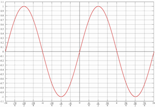
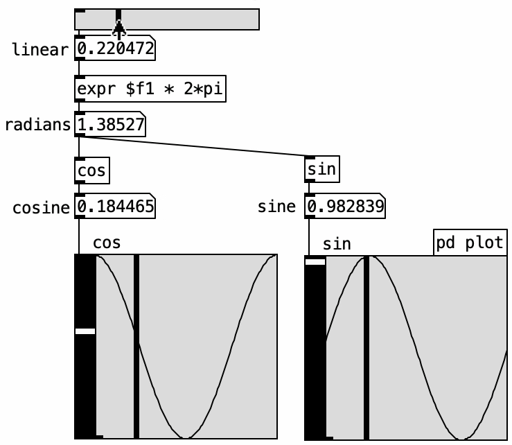
A pure tone consists of a single frequency and is produced by a sine wave oscillator, which can be implemented using either the sine or cosine function. These functions take an angle value, or “phase,” as input. Below, we see the angle “alpha,” the sine’s amplitude value, and the cosine’s output denoted as x.
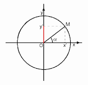
In the resulting graph, amplitude is on the vertical axis and angle on the horizontal axis. The cosine output traces the same function as the sine but starts at 1, meaning it has a different initial phase. Sine and cosine are essentially the same waveform offset by 90 degrees of phase.
Pd’s native [sin] and [cos] objects take angle values in radians \((0 \text{ to } 2\pi)\). However, the audio object [cos~] uses a linear range from 0 to 1 to represent a full cycle. The ELSE library provides the [pi] object, which outputs the constant \(\pi\). This can be stored in a [value] object and accessed within [expr]. To convert a linear 0–1 range into radians, multiply it by \(2\pi\):
\[\text{radians} = \text{linear\_input} \times 2\pi\]
Then, [cos] and [sin] yield amplitude values accordingly:
\[\text{amplitude} = \cos(\text{radians}) \text{ or } \sin(\text{radians})\]
4.2.3 Phasor
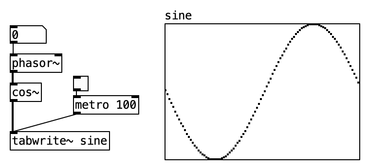
In the following example, we implement a sine oscillator using the [sin~] object and the native [phasor~] object.
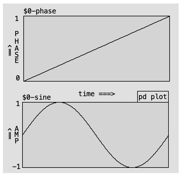
Two graphs illustrate this: in the top one, the horizontal axis is time, and the vertical axis shows a steadily increasing phase, forming a linear ramp. In the bottom graph, this ramp is transformed into a sine waveform, with amplitude on the vertical axis.
The [phasor~] object outputs a linear ramp from 0 to just under 1, representing a complete cycle. It is ideal for driving objects like [cos~] and [sin~], which expect a 0–1 input representing phase progression.
The input to [phasor~] is frequency, expressed in cycles per second (hertz). This defines how many full 0–1 cycles occur per second.
Note that [phasor~] never actually reaches 1—it wraps around to 0. Due to its cyclic nature, 1 is functionally equivalent to 0, just like 360° equals 0° in circular geometry.
The output of [phasor~] can be described as a “running phase.” It defines the angular increment applied to the phase at every audio sample.
4.2.4 Oscillator
In the analog domain, oscillators are commonly referred to as VCOs (Voltage Controlled Oscillators). VCOs allow frequency or pitch to be controlled via voltage. Some VCOs also feature voltage control inputs for modulation (typically FM) and for altering the waveform shape—usually the pulse width of square waves, although some VCOs allow shaping other waveforms as well.
Many VCOs include an additional input for synchronization with another VCO’s signal. Phase sync forces the VCO to reset its phase in sync with the incoming signal, limiting operation to harmonics of the input frequency. This results in a harsh, buzzy tone. Softer sync techniques can yield timbral variations rather than locking to an exact frequency.
A typical VCO offers controls for coarse and fine tuning, waveform selection (often sine, triangle, square, sawtooth, and pulse), pulse width modulation (PWM), and output level. Some VCOs also provide multiple simultaneous waveform outputs and sub-octave outputs one or two octaves below the main signal. Pulse width modulation (PWM) allows dynamic alteration of the pulse waveform shape.
To summarize, an oscillator is typically defined by:
- Waveform function (sine, sawtooth, square, triangle)
- Frequency (Hz)
- Initial phase (degrees)
- Peak amplitude (optional)
How do we control these parameters in our model?
4.2.5 VCO
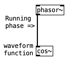
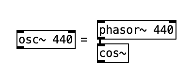
In this example, [phasor~] and [cos~] form an oscillator. The [cos~] object outputs amplitude values from -1 to 1, yielding a maximum amplitude of 1 without additional gain control.
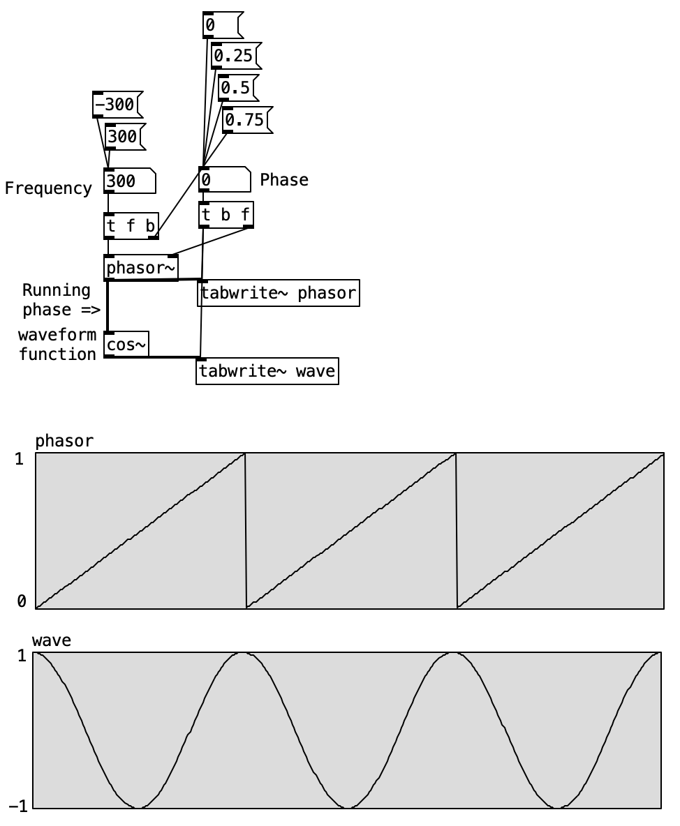
The waveform produced is a cosine. While [phasor~] sets the frequency, it can also define the initial phase. Since sine and cosine are essentially phase-shifted versions of the same function, we can easily produce sine waves as well. However, the initial phase does not affect the perceived pitch of a pure tone.
Try this patch with different phase offsets. Note that [phasor~] also accepts negative frequencies, reversing the phase direction.
Connecting [phasor~] to [cos~] replicates the functionality of the [osc~] object.
4.2.6 Waveforms
The sine wave is the simplest oscillator, generating a pure tone. Other basic and musically useful waveforms include triangle, sawtooth, and square.
The sine wave is a smooth, rounded waveform based on the sine function. It contains only one harmonic—the fundamental—which makes it less suitable for subtractive synthesis as it lacks overtones to filter.
A triangle wave consists of two linear slopes. It contains small amounts of odd harmonics, providing just enough spectral content for filtering.
A square wave contains only odd harmonics and produces a hollow, synthetic sound. A sawtooth wave contains both odd and even harmonics and sounds bright. Some pulse waves may contain even more harmonic content than basic sawtooth waves. Variants like “super-saw” replace linear slopes with exponential ones and alternate teeth with gaps, producing an even richer harmonic spectrum.
4.2.7 Waveshapers
This section focuses on creating oscillators in Pd using the [phasor~] object. The only true oscillator in Pd Vanilla is [osc~], a sine wave oscillator. Even standard waveforms must be built manually.
As mentioned earlier, [osc~] is essentially [phasor~] connected to [cos~]. The [phasor~] object outputs a 0–1 ramp, functionally similar to a sawtooth wave with half the amplitude and an offset:
\[0 \leq \text{phasor output} < 1\]
[cos~] multiplies this ramp by \(2\pi\) and computes its cosine:
\[\text{Output} = \cos(2\pi \times \text{phasor output})\]
The result is a sine wave oscillator where the complete transformation can be expressed as:
\[\begin{align*} \text{Phase} &= \text{phasor}(f) \\ \text{Sine wave} &= \cos(2\pi \times \text{Phase}) \end{align*}\]
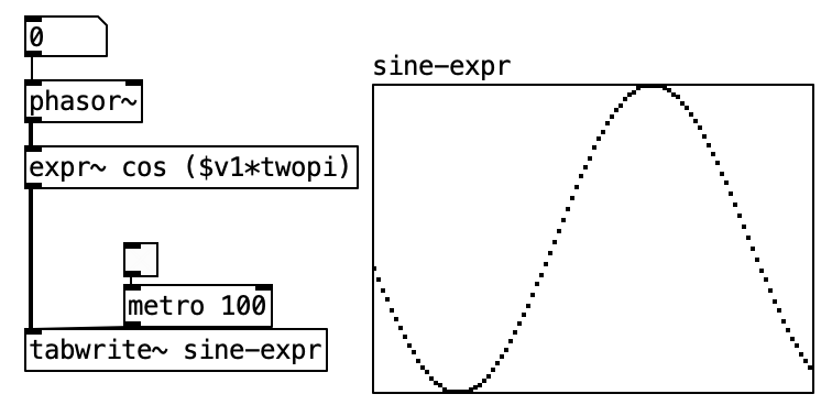
Another way to construct this oscillator is by using [expr~] and [value]. Here we use the [pi] abstraction to calculate π (or approximate it by sending 1 to [atan] and multiplying the result by 4). We then multiply by 2 and store it in a [value] object. [value] acts like a global variable: any object using the same name accesses the same value. [expr~] can then use this to calculate the cosine, just like [cos~]. While this approach may be more CPU-intensive, it helps deepen understanding of oscillator construction in Pd.
4.2.7.1 Sawtooth Oscillator
Since [phasor~] already produces a ramp, generating a sawtooth wave is straightforward. Simply multiply [phasor~] by 2 to get the correct amplitude, then subtract 1 to shift the range to -1 to 1.

4.2.7.2 Square Wave Oscillator
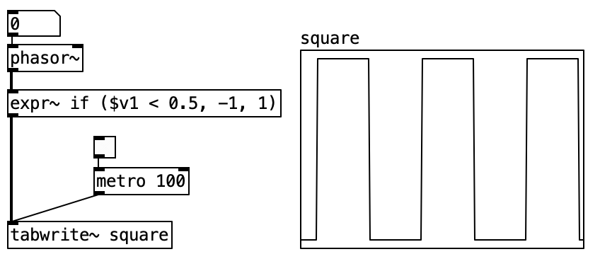
To create a square wave, you can use [expr~] (included in Pd Vanilla), but [>~] is faster and more CPU-efficient. A square wave toggles between -1 and 1. The [>~] object compares its left input signal to a threshold (right input or argument). It outputs 1 if the input is greater than the threshold, and 0 otherwise. Using 0.5 as the threshold with a [phasor~] input yields a square wave: 0 for half the cycle, 1 for the other half.
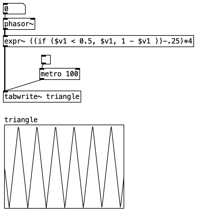
4.2.7.3 Triangle Wave Oscillator
Among standard waveforms, the triangle wave is the most complex to construct. Starting with [phasor~], which is an upward ramp from 0 to 1, we create an inverted version by multiplying it by -1 and then adding 1. This gives us a descending ramp from 1 to 0.
Now we have both ascending and descending ramps. Sending both to [min~] (which outputs the smaller of two values) gives us a triangle waveform spanning 0 to 0.5. [min~] effectively splices the ascending and descending ramps to form a symmetric triangle wave.
4.2.8 Frequency
Frequency is presented here in terms of angular velocity! One common unit of measurement is the hertz (Hz), which equals “cycles per second.” Frequency also determines a period of oscillation, which is simply the inverse of frequency. For example, a frequency of 100 Hz corresponds to a period of 0.01 seconds (or 10 milliseconds):
\[\text{Period} = \frac{1}{\text{Frequency}}\] \[\text{Period} = \frac{1}{100 \text{ Hz}} = 0.01 \text{ s} = 10 \text{ ms}\]
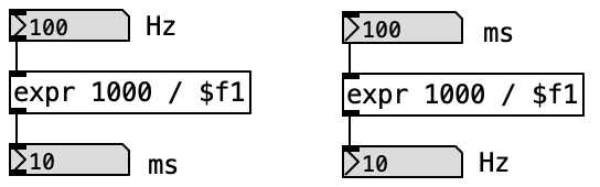
We can convert between Hz and milliseconds using this same relationship. Another way to express period is in number of samples, which requires the sampling rate to perform the conversion:
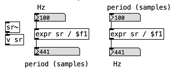
Angular velocity units require both an angle and a time unit. One cycle per second defines a full cycle (360 degrees) as the angular unit, and seconds as the time unit. Other units are also possible. For example, the angle may be expressed in radians and the time unit as a single sample, yielding a unit of “radians per sample.”
To convert Hz to radians per sample, multiply by 2π and divide by the sampling rate. See below for this conversion and the [hz2rad] and [rad2hz] objects from the ELSE library that handle it.
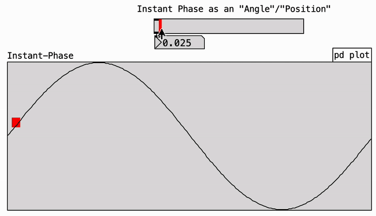
4.2.9 Phase
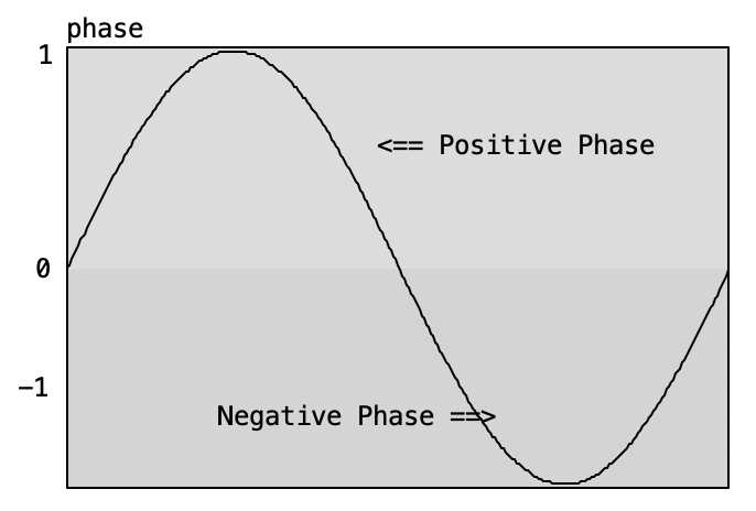
The term phase can be used in various contexts, often making it ambiguous and potentially confusing. A useful strategy is to adopt more specific terminology instead of simply referring to “phase” in isolation. On its own, “phase” refers to a stage within a cycle—much like the four phases of the moon. Sound waveforms are cyclical, and we can speak of a positive or negative phase, as shown below. However, this original meaning is rarely used in music theory. Here, we focus on other more relevant applications and interpretations of phase (see right and below).
Initial phase refers to the point in the cycle where the oscillation begins.
Instantaneous phase: In music theory, “phase” often refers to the instantaneous phase—a specific point in time, not a stage in a sequence. It’s helpful to adopt the term instantaneous explicitly to denote a single position within a given cycle.
Since instantaneous phase refers to a single position within a cycle, it can also be represented as an angle. This leads to a synonymous relationship between phase and angle, though it’s important to stress that both denote a position within the cycle.
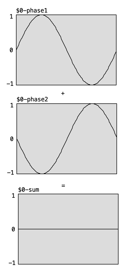
Two oscillators operating at the same frequency can be in phase or out of phase. Being in phase means they are synchronized—there is no phase difference. Being out of phase indicates a lack of synchronization, i.e., a phase difference. This difference can take many forms, but two specific cases are of particular interest: quadrature phase and phase opposition.
Quadrature phase is the phase difference between sine and cosine waves, which equals a quarter of a cycle (90 degrees).
Phase opposition is the maximum possible phase difference—half a cycle or 180 degrees.
4.2.10 Polarity
As we’ve seen, phase opposition leads to signal cancellation—but only under certain waveform conditions! This occurs with sine waves, for instance, but not with all waveforms or signals. Note how, in the figure to the right, inverting the sign of every amplitude value in a waveform results in cancellation when added to the original signal.
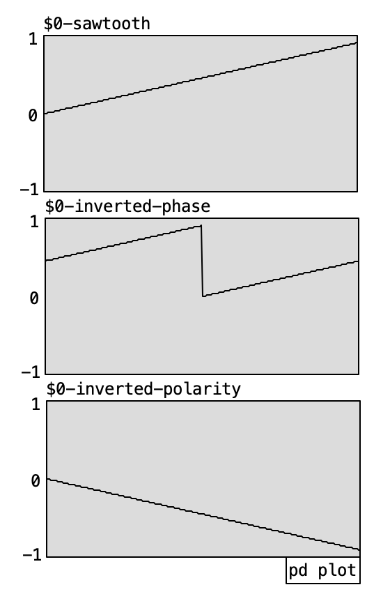
Inverting polarity means changing the sign, or multiplying by -1. For sine waves, this results in the same effect as a 180-degree phase opposition. However, a true phase inversion is different, as it involves a time or phase shift.
Despite this distinction, the term phase inversion is often misused when it really refers to a polarity inversion—which is neither a time shift nor a phase shift.
Yes, this can be very confusing and requires careful attention. That’s why this tutorial prefers the term polarity inversion, although many audio devices refer to a 180-degree phase shift when they are, in fact, performing a polarity inversion.
Both phase and polarity inversion produce the same result for sine waves due to their symmetrical waveforms, where the second half of the cycle mirrors the first with opposite sign. Other waveforms with this property include triangle and square waves (with a 0.5 pulse width).
Sawtooth waves, however, do not share this symmetry. Therefore, phase opposition is not equivalent to polarity inversion in this case. The only way to achieve full cancellation of a sawtooth wave is through polarity inversion. Refer to the graphs below: only the original sawtooth combined with its polarity-inverted version results in complete cancellation.
The native [phasor~] and [osc~] objects include a right inlet that accepts control data to reset the phase. Whenever the inlet receives a number from 0 to 1, the waveform resets to that initial phase position. Note that this is unrelated to phase modulation techniques discussed earlier.
The [osc~] object does not support phase modulation; we implemented it using [phasor~] in the previous examples. Hence, using a [phasor~] together with a [cos~] enables both phase modulation and oscillator resetting.
4.3 Additive Synthesis
Additive synthesis is a method for constructing complex waveforms by combining multiple sine waves of different frequencies and amplitudes. Unlike subtractive synthesis, which begins with a harmonically rich signal and removes unwanted components through filtering, additive synthesis starts from fundamental building blocks—sine waves—and gradually assembles them into a desired sound. While the conceptual clarity of this approach is appealing, its practical implementation typically demands a user interface capable of managing a high number of parameters simultaneously, often making additive synthesizers more complex to operate.
The theoretical foundation of additive synthesis lies in the work of the French mathematician Jean-Baptiste Joseph Fourier. In 1807, Fourier demonstrated that any periodic waveform could be represented as a sum of sine waves, each with a specific frequency and amplitude. This revelation forms the basis of what we now call Fourier analysis and synthesis. While Fourier’s original formulation applied only to repetitive waveforms to maintain mathematical tractability, modern techniques extend these principles to non-periodic signals by allowing sine wave parameters to vary over time.
A helpful analogy is to imagine describing written text over a telephone to someone who has never seen it. One might begin by breaking words into letters, and letters into lines, curves, and dots. This level of description works well if the words remain static. However, if the words change, the description must be updated continuously. Likewise, Fourier synthesis allows us to describe and reproduce complex waveforms from basic sinusoidal components, provided we are equipped to update these components when the signal changes.
The simplest application of Fourier synthesis is the reconstruction of a sine wave—which, unsurprisingly, requires just one sine wave. A sine wave contains only a single frequency component—the fundamental—and no additional harmonics.
4.3.1 Harmonics and Waveform Construction
More complex waveforms are created by adding sine waves at integer multiples of the fundamental frequency. These multiples are called harmonics. If the fundamental frequency is denoted by ( f ), then the additional components will be ( 2f, 3f, 4f, ), corresponding to the second, third, fourth harmonics, and so on. This organization gives rise to the standard harmonic series found in many acoustic and electronic sounds.
The terminology surrounding harmonics often overlaps with that of overtones. The first harmonic (fundamental) has no overtone. The second harmonic is the first overtone, the third harmonic is the second overtone, and so forth. This relationship is summarized in the following table:
| Frequency | Harmonic | Overtone |
|---|---|---|
| ( f ) | 1 | — |
| ( 2f ) | 2 | 1 |
| ( 3f ) | 3 | 2 |
| ( 4f ) | 4 | 3 |
| ( 5f ) | 5 | 4 |
| ( 6f ) | 6 | 5 |
| ( 7f ) | 7 | 6 |
| ( 8f ) | 8 | 7 |
| ( 9f ) | 9 | 8 |
| ( 10f ) | 10 | 9 |
4.3.2 Harmonic Synthesis
Although additive synthesis often begins with the goal of reconstructing a known waveform, this is a limited perspective. In practice, the visual shape of a waveform does not reliably indicate its harmonic content. Minor alterations in phase relationships can drastically alter the shape of a waveform without affecting its sonic character. This is especially true at higher frequencies, where the human auditory system is less sensitive to phase differences.
For example, sine waves are considered perceptually pure. Introducing odd-numbered harmonics yields a triangular waveform, which retains a clean quality but feels richer than a pure sine. Square waves contain only odd harmonics, lending them a hollow timbre. If the second harmonic of a square wave is phase-shifted, the visual waveform changes, yet the auditory perception remains largely unaffected. Sawtooth waves, containing both even and odd harmonics, are brighter and richer in harmonic content. Modifying the phase of their components alters the shape without significantly changing the perceived sound.
Pulse waves, derived from narrow square waves, introduce more harmonics as the duty cycle deviates from 50%. Interestingly, a 10% and a 90% pulse wave share identical harmonic content, illustrating the symmetry of their spectrum. The square wave (50% duty cycle) is unique in that it contains only odd harmonics. By contrast, a waveform composed exclusively of even harmonics resembles a square wave shifted up by an octave—its fundamental frequency is ( 2f ).
4.3.3 Practical Considerations
Perfect waveforms, such as ideal square waves, require an infinite number of harmonics. In practice, synthesizers approximate these shapes with a limited set of partials, usually between 32 and 64 harmonics. For instance, a fundamental frequency of 55 Hz (low A) yields the 32nd harmonic at 1760 Hz and the 64th at 3520 Hz. At 440 Hz (concert A), the 45th harmonic reaches 19,800 Hz, which is near the upper limit of human hearing.
| Frequency | Harmonic |
|---|---|
| 55 Hz | 1 |
| 110 Hz | 2 |
| 165 Hz | 3 |
| 220 Hz | 4 |
| 275 Hz | 5 |
| … | … |
| 3520 Hz | 64 |
4.3.4 Inharmonic Content and Real-World Complexity
Real-world sounds often exhibit inharmonic components—frequencies that are not integer multiples of the fundamental. These include:
- Noise: Broad-spectrum energy with no harmonic organization.
- Beat Frequencies: Resulting from detuned harmonics, producing low-frequency amplitude modulations.
- Sidebands: Occurring from modulation, producing spectral mirror images around a carrier frequency.
- Inharmonics: Regularly structured but non-harmonic components, typical of metallic or bell-like sounds.
Many additive synthesizers limit themselves to harmonic content, occasionally supplemented by noise generators. While deterministic in design, this approach overlooks the stochastic and dynamic nature of real-world sound phenomena.
4.3.5 Harmonic Analysis
To construct realistic timbres, additive synthesis relies on knowledge of harmonic spectra from real instruments. Fourier analysis provides a systematic method for decomposing complex signals into their constituent sine waves. This is conceptually akin to sweeping a narrow band-pass filter across the spectrum and measuring energy at each frequency. The narrower the filter bandwidth, the higher the resolution. Simple musical tones require relatively coarse resolution; more complex sounds demand finer spectral discrimination.
Fourier analysis can be performed with analog hardware or more commonly with digital processing techniques, offering flexibility and precision for real-time applications.
4.3.6 Envelopes in Additive Synthesis
Controlling the amplitude of each harmonic over time requires an envelope generator (EG) and a voltage-controlled amplifier (VCA) per harmonic. Ideally, the final sound envelope results from the sum of individual harmonic envelopes. To simplify control while preserving expressivity, a global EG and VCA can also be applied post-summing to modulate the overall output.
One common configuration is the ADSR envelope—Attack, Decay, Sustain, Release—which requires only four parameters and is relatively easy to implement in analog circuitry. Though more complex designs like DADSR offer additional flexibility, they demand more components and are usually reserved for digital implementations.

Additive synthesis provides a powerful framework for sound construction, especially when paired with modern computational tools. It invites a deep understanding of harmonic behavior and spectral composition, allowing composers and designers to sculpt timbre with surgical precision—layer by layer, sine by sine.
The following example created by Miller Puckette (Puckette 2007) encapsulate an ADSR envelope generator within a reusable Pd abstraction named adsr. This design enables easy replication of the envelope generator and flexible parameter control, either through creation arguments or real-time updates via control inlets.
The abstraction accepts five creation arguments, corresponding respectively to the:
- peak level
- attack time
- decay time
- sustain level (expressed as a percentage of the peak), and
- release time
For instance, the arguments [adsr 1 100 200 50 300] define a peak amplitude of 1.0, an attack time of 100 milliseconds, a decay time of 200 milliseconds, a sustain level at 50% of the peak, and a release time of 300 milliseconds.
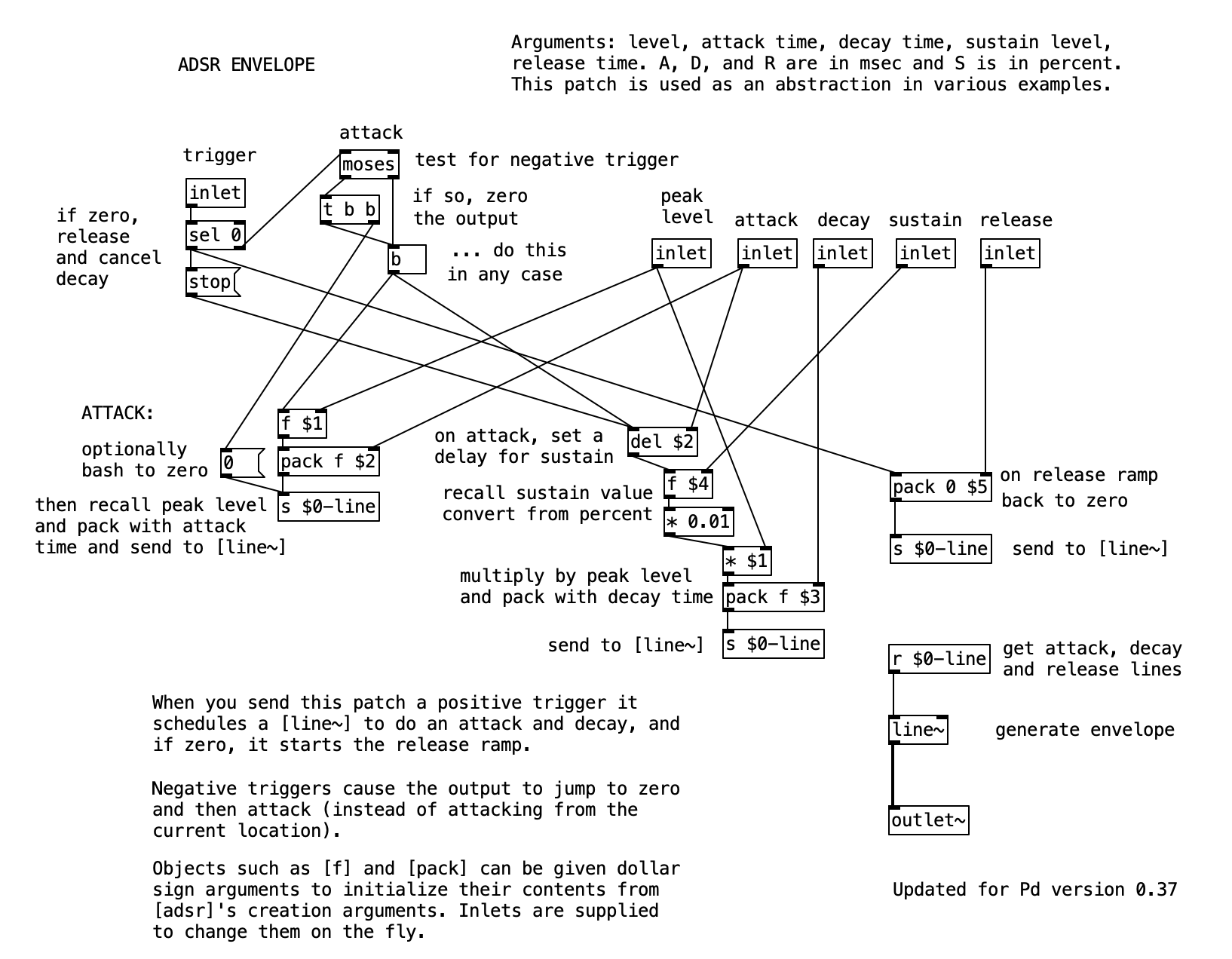
In addition to these arguments, the abstraction provides six control inlets. The first inlet serves as the trigger input, responsible for initiating or releasing the envelope. The remaining five inlets allow dynamic control over each of the ADSR parameters, overriding the corresponding creation arguments when values are received. The abstraction outputs an audio signal that modulates amplitude according to the ADSR envelope.
Internally, the implementation of the adsr abstraction is both efficient and modular. The signal path consists of the standard [line~] object, used to generate smooth audio ramps, and [outlet~], which delivers the envelope signal to the external patch. Control flow within the abstraction is handled through three [pack] objects—each corresponding to a message that controls one segment of the envelope: attack, decay, and release.
The attack segment uses a [pack] object to format a message that instructs [line~] to ramp from 0 to the peak level over the attack time duration. This peak level is represented by $1, the first creation argument, while the duration is $2, the second. Both values can also be modified via the corresponding control inlets.
The decay segment presents a more complex behavior. Once the attack segment is completed, the envelope should transition from the peak to the sustain level. This transition is delayed using [del $2], which defers execution by the duration of the attack. The sustain level is computed by multiplying the peak value by the sustain percentage (the fourth creation argument or inlet), and dividing by 100. This result becomes the new target value for [line~], reached over the duration specified by the decay time.
The release segment is comparatively straightforward. Upon receiving a trigger value of 0, the abstraction sends a ramp to zero over the specified release time. This is implemented using a [pack] object that combines the zero target with the release time value, which is either $5 (from creation arguments) or provided via the corresponding inlet.
The trigger logic supports three types of behavior:
- A positive number initiates an attack and decay cycle.
- A zero triggers the release segment, allowing the envelope to fade back to zero.
- A negative number functions as a reset, immediately sending the output to zero and initiating a new onset.
This flexibility enables the abstraction to support a variety of amplitude modulation scenarios in real-time audio synthesis, making it both pedagogically instructive and practically versatile for sound design tasks.
4.3.7 Twenty-Oscillator Harmonic System
This Pd patch implements a comprehensive additive synthesis engine that shows the fundamental principles of harmonic spectrum construction through the controlled combination of multiple sine wave oscillators. The system employs twenty independent oscillator modules, each operating at harmonically related frequencies with individual amplitude envelope control, creating a powerful platform for exploring the timbral possibilities of additive synthesis while maintaining real-time performance capabilities.
The patch architecture emphasizes modular design through the use of custom abstractions, enabling scalable harmonic control while providing educational insight into the mathematical relationships that govern harmonic series construction. By implementing individual envelope generators for each partial, the system demonstrates how complex timbral evolution can be achieved through coordinated amplitude control across multiple frequency components.
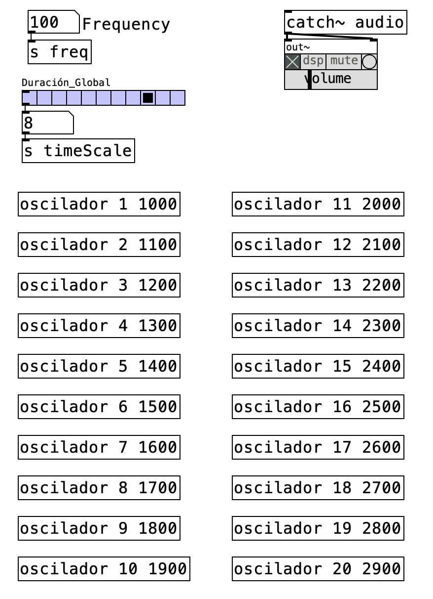
4.3.7.1 Patch Overview
The additive synthesis system implements a comprehensive harmonic generation pipeline consisting of four primary processing stages:
- Global Parameter Control: Manages fundamental frequency and timing coordination
- Individual Oscillator Modules: Twenty independent
osciladorabstractions with harmonic frequency relationships - Amplitude Envelope Management: Coordinated envelope generation across all partials
- Audio Signal Summation: Collection and mixing of all oscillator outputs
The system demonstrates classic additive synthesis principles where complex timbres emerge from the controlled combination of simple sinusoidal components, each contributing specific harmonic content to the overall spectral composition.
4.3.7.2 Critical Processing Components
oscilador Abstraction: Each instance implements a complete harmonic partial with integrated envelope generation. The abstraction receives two arguments: harmonic number (1-20) and envelope duration in milliseconds, enabling independent control over both frequency relationships and temporal characteristics.
Global Parameter Distribution: The send/receive system (s freq, s timeScale) ensures synchronized parameter updates across all oscillator instances while maintaining modular architecture that supports easy scaling to different numbers of partials.
Audio Signal Aggregation: The catch~ audio object employs Pd’s audio signal collection mechanism to sum all oscillator outputs without explicit connection cables, demonstrating efficient signal routing in complex patches.
4.3.7.3 Data Flow
The additive synthesis patch orchestrates a multi-oscillator system that transforms simple frequency and timing parameters into complex harmonic spectra through coordinated oscillator management and envelope control. This implementation demonstrates how additive synthesis principles can be systematically applied to create timbral complexity from elementary sinusoidal components while maintaining real-time performance and user control.
The global parameter management stage establishes the foundation for harmonic spectrum generation through centralized control of fundamental frequency and timing coordination. When users adjust the frequency control, the new value propagates through the s freq send object to all twenty oscillator instances simultaneously, ensuring that harmonic relationships remain mathematically correct as the fundamental frequency changes. This distribution system maintains the precise frequency ratios that define harmonic series relationships, where each oscillator operates at an integer multiple of the fundamental frequency. The timing control system operates in parallel through the s timeScale, enabling users to adjust the overall temporal character of the synthesis while preserving the relative envelope timing relationships between different partials. The hradio interface provides discrete envelope duration options that range from brief percussive attacks to sustained harmonic evolutions, allowing for diverse timbral expressions within the additive framework.
The individual oscillator processing stage represents the core of the additive synthesis engine, where each oscilador abstraction implements a complete harmonic partial with sophisticated envelope control. Each oscillator instance receives two critical arguments during instantiation: the harmonic number (1, 2, 3… up to 20) and the base envelope duration in milliseconds. The harmonic number determines the frequency multiplication factor applied to the global fundamental frequency, creating the precise integer relationships that define harmonic spectra. Within each oscilador abstraction, the frequency calculation multiplies the received fundamental frequency by the harmonic number, generating frequencies such as 440 Hz (fundamental), 880 Hz (second harmonic), 1320 Hz (third harmonic), and so forth. The envelope duration argument provides each oscillator with its temporal characteristics, which are further modified by the global time scaling factor to enable coordinated timing adjustments across the entire harmonic spectrum.
The envelope generation and coordination stage implements sophisticated temporal control that enables complex timbral evolution through coordinated amplitude modulation across all harmonic partials. Each oscilador abstraction contains an independent envelope generator that controls the amplitude trajectory of its associated sine wave oscillator. The envelope system employs bang-triggered activation that initiates synchronized envelope sequences across all oscillators, creating coherent timbral attacks and evolutions. The envelope duration calculation combines the base duration argument with the global time scaling factor, enabling users to modify the overall temporal character of the synthesis while maintaining the relative timing relationships between different partials. This coordination mechanism allows for sophisticated timbral effects where lower harmonics might sustain longer than higher harmonics, or where specific partials activate at different times to create complex spectral evolution patterns.
The audio signal collection and output stage demonstrates efficient signal routing architecture that aggregates all oscillator outputs without requiring complex cable connections between modules. Each oscilador abstraction contains a throw~ audio object that sends its processed audio signal to the global collection point implemented by the catch~ audio object in the main patch. This signal routing approach enables the system to sum all twenty harmonic partials automatically while maintaining clean patch organization and supporting easy modification of the oscillator count. The collected audio signal undergoes final processing through the out~ object, which provides level control and audio interface connectivity for monitoring and recording the synthesized output.
flowchart LR
    A[Parameter Distribution] --> B[Harmonic Generation]
    B --> C[Envelope Application]
    C --> D[Signal Collection]
4.3.7.4 Processing Chain Details
The additive synthesis system maintains harmonic precision and temporal coordination through several interconnected processing stages:
| Stage | Input | Process | Output |
|---|---|---|---|
| 1 | User Controls | Global parameter distribution | Synchronized frequency and timing |
| 2 | Global Parameters | Harmonic frequency calculation | Twenty harmonic frequencies |
| 3 | Harmonic Frequencies | Sine wave generation with envelopes | Individual partial signals |
| 4 | Multiple Audio Signals | Signal aggregation and mixing | Combined harmonic spectrum |
4.3.7.5 Harmonic Frequency Distribution
| Oscillator | Harmonic Number | Frequency Relationship | Example (440 Hz fundamental) |
|---|---|---|---|
| 1 | 1 | f × 1 | 440 Hz |
| 2 | 2 | f × 2 | 880 Hz |
| 3 | 3 | f × 3 | 1320 Hz |
| 4 | 4 | f × 4 | 1760 Hz |
| 5 | 5 | f × 5 | 2200 Hz |
| 6-10 | 6-10 | f × 6-10 | 2640-4400 Hz |
| 11-15 | 11-15 | f × 11-15 | 4840-6600 Hz |
| 16-20 | 16-20 | f × 16-20 | 7040-8800 Hz |
4.3.7.6 Envelope Timing Control
The time scaling system provides proportional control over envelope durations:
| hradio Setting | Time Scale Factor | Effect on 1000ms Base Duration |
|---|---|---|
| 0 | 0.1 | 100 ms (very fast attack) |
| 1 | 0.25 | 250 ms (fast attack) |
| 2 | 0.5 | 500 ms (medium attack) |
| 3 | 1.0 | 1000 ms (normal attack) |
| 4 | 2.0 | 2000 ms (slow attack) |
| 5 | 5.0 | 5000 ms (very slow attack) |
4.3.7.7 Signal Architecture
Modular Design: Each oscillator operates independently while sharing global parameters, enabling flexible harmonic control and easy system modification.
Efficient Routing: The throw/catch system eliminates cable clutter while maintaining clear signal flow organization.
Scalable Architecture: The abstraction-based design supports easy addition or removal of harmonic partials without patch restructuring.
4.3.7.8 Key Objects and Their Roles
| Object | Function | Role in Additive Synthesis |
|---|---|---|
s freq / r freq |
Global frequency distribution | Distributes fundamental frequency to all oscillators |
oscilador |
Harmonic oscillator abstraction | Implements individual partial with envelope control |
catch~ audio |
Audio signal collection | Aggregates all oscillator outputs |
s timeScale / r timeScale |
Timing distribution | Coordinates envelope durations across oscillators |
out~ |
Audio output | Final signal delivery |
4.3.7.9 Creative Applications
- Classic Additive Synthesis: Recreate the timbres of historical additive synthesizers like the Kawai K5000 or early computer music systems by manually adjusting individual harmonic amplitudes
- Spectral Animation: Use external control data (MIDI, OSC, sensors) to modulate individual oscillator amplitudes, creating dynamic spectral evolution and movement
- Organ Stop Simulation: Configure different combinations of harmonics to simulate pipe organ stops, drawbar organs, or other harmonic instruments
- Spectral Morphing: Sequence different harmonic amplitude configurations to create smooth timbral transitions between distinct spectral shapes
- Microtonal Additive Synthesis: Modify individual oscillator frequencies to explore non-harmonic spectra and microtonal intervals while maintaining the additive framework
- Algorithmic Composition: Use mathematical functions or stochastic processes to control harmonic amplitudes over time, creating evolving textures with embedded structural logic
4.3.8 Additive Clone: Scalable Harmonic Synthesis
This Pd patch implement a dynamic additive synthesis using Pd’s clone object to create a scalable system of harmonic oscillators. Unlike fixed multi-oscillator systems, this implementation allows real-time adjustment of the number of active partials, from 1 to 20, while maintaining proper amplitude scaling to prevent clipping. The patch showcases advanced Pd programming techniques including dynamic object creation, parameter distribution, and automatic scaling based on psychoacoustic principles.
The system emphasizes efficiency and modularity by using identical harmonic abstractions that receive initialization parameters and operate independently. This approach enables exploration of how partial count affects timbral complexity while demonstrating the relationship between harmonic density and perceived loudness.
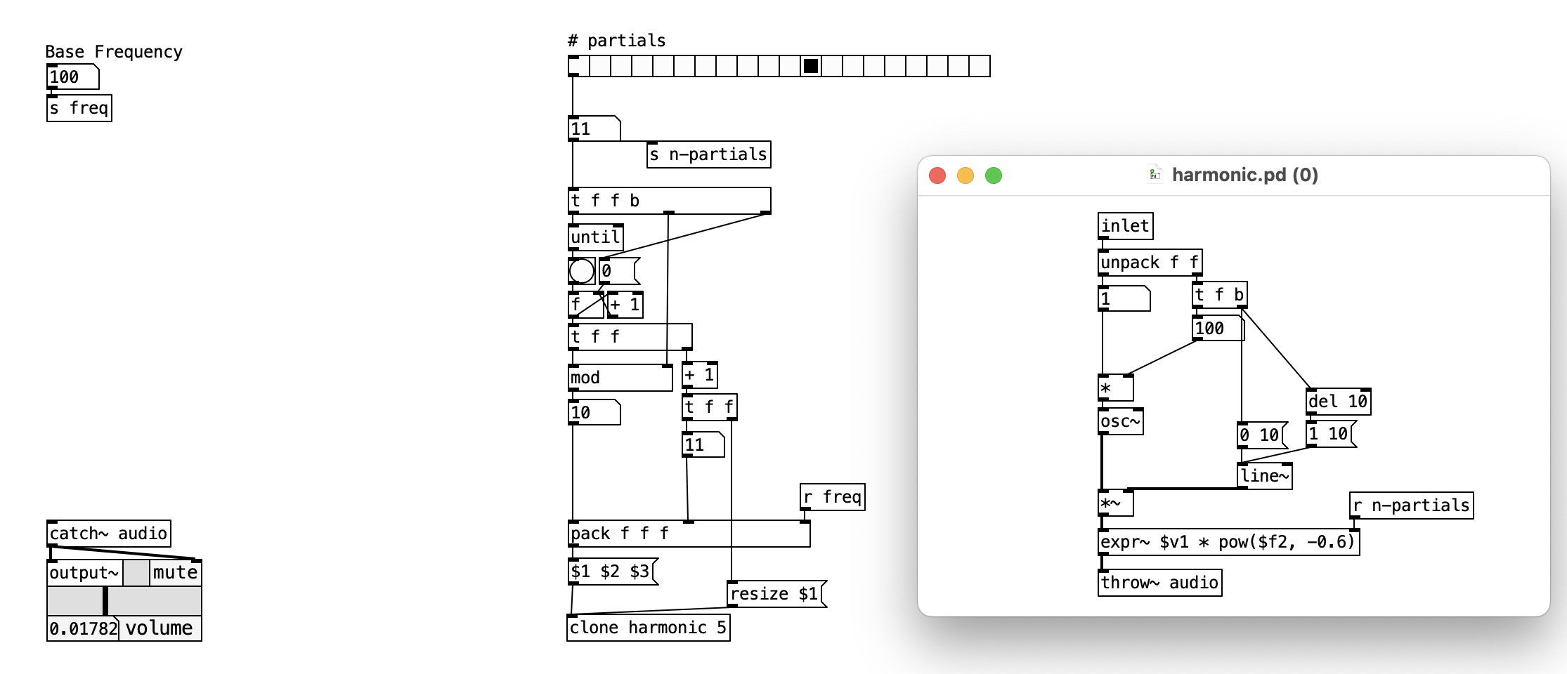
4.3.8.1 Patch Overview
The additive clone system implements a dynamic harmonic generation pipeline consisting of four primary processing stages:
- Partial Count Control: Interface for selecting number of active harmonics (1-20)
- Parameter Generation: Algorithmic calculation of frequency multipliers and amplitude coefficients
- Dynamic Instance Management: Clone-based creation of harmonic oscillators with scaling
- Audio Collection: Signal aggregation with psychoacoustic amplitude compensation
The patch demonstrates how algorithmic parameter generation can control large numbers of synthesis components while maintaining musical coherence and preventing amplitude overflow.
4.3.8.2 Critical Dynamic Components
Clone Object Management: The clone harmonic object dynamically creates instances based on the resize message, enabling real-time adjustment of synthesis complexity without patch reconstruction.
Psychoacoustic Scaling: The expr~ pow($f2, -0.6) calculation in each harmonic applies amplitude reduction based on the total number of active partials, using research-based scaling that matches human loudness perception.
Modular Parameter Generation: The until and mod system creates a counting sequence that generates unique harmonic numbers for each clone instance while handling array wraparound.
4.3.8.3 Data Flow
flowchart TD
    A[Partial Count Selection] --> B[Parameter Generation Loop]
    B --> C[Clone Instance Creation]
    C --> D[Individual Harmonic Processing]
    D --> E[Amplitude Scaling]
    E --> F[Audio Collection]
    F --> G[Mixed Output]

    style A fill:#e1f5fe
    style G fill:#f3e5f5
    style E fill:#fff3e0
The additive clone patch implmenting a dynamic synthesis system that adapts the number of active harmonic oscillators in real-time while maintaining proper amplitude relationships and preventing audio clipping. This implementation demonstrates how Pd’s clone object can be combined with algorithmic parameter generation to create scalable synthesis systems that remain musically coherent across different levels of harmonic complexity.
The partial count control stage establishes the foundation for dynamic synthesis through user interface management that directly controls system complexity. The hradio interface enables selection of partial counts from 1 to 20, with each selection triggering a complete reconfiguration of the synthesis system. The selected value propagates through two parallel pathways: immediate distribution via the s n-partials send system that informs all existing harmonic instances of the new partial count, and initiation of the parameter generation sequence that calculates appropriate settings for the requested number of oscillators. This dual distribution ensures that both the scaling calculations within individual harmonics and the overall system configuration remain synchronized as users adjust the synthesis complexity in real-time.
The algorithmic parameter generation stage transforms the simple partial count selection into comprehensive initialization data for each harmonic oscillator through systematic mathematical processing. The until object creates an iteration loop that executes the specified number of times, generating unique parameter sets for each harmonic instance. During each iteration, the counter value undergoes processing through the mod object, which provides frequency multiplier values that cycle through a predetermined sequence, enabling harmonic relationships that extend beyond simple integer multiples if desired. The counter value also serves directly as the harmonic number identifier, while the fundamental frequency received through r freq provides the base frequency reference. These three values combine in the pack f f f object to create complete initialization messages that contain all information necessary for each harmonic instance to configure its frequency relationships and amplitude characteristics.
The dynamic instance management stage demonstrates Pd’s advanced object creation capabilities through an implementation of the clone system that adapts to changing synthesis requirements. When the resize message reaches the clone harmonic object, it dynamically adjusts the number of active harmonic instances, creating new oscillators when the count increases or deactivating instances when the count decreases. Each parameter pack message generated by the algorithmic calculation stage initializes a harmonic instance with its specific frequency multiplier and amplitude coefficient. The clone system manages this distribution automatically, ensuring that each active instance receives appropriate initialization data while maintaining efficient resource utilization. This dynamic approach enables the system to scale from simple single-oscillator tones to complex 20-partial harmonic spectra without requiring manual patch reconfiguration or predetermined oscillator allocation.
The individual harmonic processing stage occurs within each harmonic abstraction instance, where distributed parameters control sophisticated oscillator and envelope systems enhanced with automatic amplitude scaling. Each harmonic receives its frequency multiplier through the initialization message and combines it with the global fundamental frequency to generate its specific harmonic frequency. The critical innovation within each harmonic involves the expr~ pow($f2, -0.6) calculation that applies amplitude scaling based on the total number of active partials received through the r n-partials system. This scaling factor implements psychoacoustic research that shows how human loudness perception requires amplitude reduction as the number of harmonic components increases, preventing the perception of increased loudness as synthesis complexity grows. The power law exponent of -0.6 provides a compromise between mathematical precision and musical utility, ensuring that 20-partial synthesis produces manageable amplitude levels while maintaining sufficient dynamic range for musical expression.
flowchart LR
    A[Partial Selection] --> B[Dynamic Configuration]
    B --> C[Scaled Audio Output]
4.3.8.4 Processing Chain Details
The dynamic additive synthesis design maintains musical coherence through coordinated processing stages:
| Stage | Input | Process | Output |
|---|---|---|---|
| 1 | User Selection | Partial count validation and distribution | System reconfiguration triggers |
| 2 | Partial Count | Iterative parameter calculation | Harmonic initialization data |
| 3 | Parameter Messages | Dynamic clone instance management | Active harmonic oscillators |
| 4 | Instance Configuration | Individual harmonic synthesis with scaling | Amplitude-compensated audio |
| 5 | Scaled Audio Streams | Signal collection and mixing | Balanced harmonic spectrum |
4.3.8.4.1 Scaling Factor Analysis
The psychoacoustic amplitude scaling prevents clipping while maintaining perceptual balance:
| Active Partials | Scaling Factor | Individual Amplitude | Perceptual Effect |
|---|---|---|---|
| 1 | 1.000 | 100% | Full single-tone amplitude |
| 5 | 0.315 | 31.5% | Balanced complex tone |
| 10 | 0.200 | 20.0% | Rich harmonic spectrum |
| 15 | 0.151 | 15.1% | Dense harmonic texture |
| 20 | 0.122 | 12.2% | Maximum complexity without clipping |
4.3.8.5 Clone Abstraction Architecture
Dynamic Scalability: Easy modification of maximum partial count through hradio range adjustment.
Efficient Resource Management: Inactive instances consume minimal CPU resources.
Parameter Synchronization: Automatic distribution of configuration changes to all active instances.
Amplitude Safety: Built-in scaling prevents output clipping across all partial count settings.
4.3.8.6 Key Objects and Their Roles
| Object | Function | Role in Dynamic Synthesis |
|---|---|---|
clone harmonic |
Dynamic instance manager | Creates variable number of oscillator instances |
until |
Parameter loop generator | Executes calculation sequence for each partial |
mod |
Frequency calculation | Generates harmonic number sequence |
expr~ pow($f2, -0.6) |
Amplitude scaling | Prevents clipping using psychoacoustic scaling |
s n-partials / r n-partials |
Partial count distribution | Distributes active partial count to all instances |
4.3.8.7 Creative Applications
- Real-time Timbral Morphing: Automate the partial count using LFOs or envelopes to create evolving timbres that transition between simple and complex harmonic structures
- Interactive Spectral Control: Map external controllers or sensors to the partial count parameter, enabling performers to sculpt harmonic complexity through gesture or movement
- Spectral Analysis Tools: Use the system to reconstruct and study natural instrument timbres by adjusting partial counts to match analyzed harmonic content
4.3.9 Spectral Melody
This patch implements an additive synthesis system that demonstrates how harmonic partial generation can be controlled through algorithmic distribution and temporal sequencing. By utilizing Pd’s clone object to create eight instances of a partial abstraction, the system generates complex harmonic spectra where each partial operates with independent amplitude envelopes and frequency relationships. The patch emphasizes real-time control over both spectral content and temporal evolution, creating a platform for exploring the relationship between harmonic structure and melodic perception.
The implementation showcases advanced Pd programming techniques including dynamic object creation, parameter distribution through send/receive networks, and sophisticated envelope generation that enables complex spectral animation. By combining systematic harmonic relationships with stochastic envelope timing, the patch creates evolving textures that bridge the gap between traditional additive synthesis and contemporary algorithmic composition.

4.3.9.1 Patch Overview
The patch implements a comprehensive harmonic generation pipeline consisting of five primary processing stages:
- Parameter Management: Global frequency and timing control with user interface
- Algorithmic Partial Distribution: Mathematical calculation of harmonic relationships and amplitude scaling
- Dynamic Synthesis Engine: Eight-instance clone system for parallel partial generation
- Stochastic Envelope Control: Randomized attack and decay timing for each partial
- Audio Collection and Output: Signal aggregation and final audio delivery
The patch demonstrates how mathematical relationships can be embedded within musical structures, where harmonic series principles guide frequency distribution while algorithmic processes control temporal evolution and spectral dynamics.
4.3.9.2 Critical Algorithmic Components
Clone Object Architecture: The clone partial 8 object creates eight independent instances of the partial abstraction, each receiving unique initialization parameters. This approach enables parallel processing while maintaining individual control over each harmonic component.
Mathematical Amplitude Distribution: The expression (8 - $f1)/8 implements inverse amplitude scaling where lower harmonics receive higher amplitudes, following natural harmonic decay patterns found in acoustic instruments.
Parameter Pack System: The pack f f f object bundles harmonic number, frequency multiplier, and amplitude coefficient into a unified message that initializes each partial instance with its specific characteristics.
4.3.9.3 Data Flow
flowchart TD
    A[User Controls] --> B[Parameter Distribution]
    B --> C[Algorithmic Calculation]
    C --> D[Clone Instance Generation]
    D --> E[Individual Partial Processing]
    E --> F[Stochastic Envelope Control]
    F --> G[Audio Collection]
    G --> H[Mixed Output]

    style A fill:#e1f5fe
    style H fill:#f3e5f5
    style C fill:#fff3e0
    style F fill:#fff3e0
The spectral melody patch implement an algorithmic synthesis process that transforms simple user parameters into complex harmonic spectra through systematic mathematical calculations and dynamic object instantiation. This implementation demonstrates how Pd’s cloning capabilities can be combined with algorithmic parameter generation to create scalable additive synthesis systems that maintain both mathematical precision and timbral expressivity.
The parameter initialization and distribution stage establishes the foundation for the entire synthesis process through coordinated management of fundamental frequency and timing parameters. When users adjust the frequency slider, the new value propagates through the s root-freq send object to all active partial instances, ensuring that harmonic relationships remain mathematically correct as the fundamental frequency changes. The duration control system operates in parallel, with the time slider feeding the s total-time distribution network that coordinates envelope timing across all eight partials. The bang trigger initiates the algorithmic calculation sequence that generates the specific parameters needed for each partial instance, creating a synchronized parameter update system that maintains harmonic coherence while enabling real-time musical control. This distribution architecture ensures that all synthesis components receive updated parameters simultaneously, preventing temporal misalignment that could compromise the spectral integrity of the additive synthesis process.
The algorithmic parameter generation stage represents the mathematical core of the system, where simple counting operations become sophisticated harmonic calculations through coordinated processing chains. The until object creates an iteration loop that executes eight times, with each iteration generating the specific parameters needed for one partial instance. During each iteration, the counter value undergoes multiple simultaneous calculations: direct passage as the harmonic number, incrementation by one to create the frequency multiplier, and processing through the amplitude calculation expression (8 - $f1)/8 to generate amplitude coefficients that follow natural harmonic decay patterns. This mathematical approach ensures that the first partial operates as the fundamental with maximum amplitude, while subsequent partials represent increasingly higher harmonics with proportionally reduced amplitudes. The pack f f f object collects these three calculated values into a unified parameter message that contains all information necessary for initializing each partial instance with its unique harmonic characteristics.
The dynamic synthesis instantiation stage demonstrates Pd’s advanced object creation capabilities through the sophisticated implementation of the clone partial 8 object. Each parameter pack message generated by the algorithmic calculation stage triggers the creation and initialization of a partial instance with specific harmonic characteristics. The clone object manages eight independent instances of the partial abstraction, distributing the parameter messages to initialize each instance with its unique harmonic number, frequency multiplier, and amplitude coefficient. This distribution process creates a parallel processing architecture where eight independent synthesis units operate simultaneously, each contributing a specific harmonic component to the overall spectral composition. The modular design enables easy scaling to different numbers of partials by simply modifying the clone argument, demonstrating the flexibility inherent in this approach to additive synthesis system design.
The individual partial processing stage occurs within each partial abstraction instance, where the distributed parameters control sophisticated oscillator and envelope systems that generate the actual harmonic content. Each partial receives the global root frequency through the receive system and multiplies it by its assigned frequency multiplier to generate its specific harmonic frequency. The amplitude coefficient controls the maximum level for that partial’s envelope system, while the total time parameter influences the temporal characteristics of the amplitude envelope. Within each partial, stochastic processes introduce controlled randomization into the envelope timing, creating complex temporal relationships between different harmonics that evolve organically over time. This combination of deterministic harmonic relationships with stochastic temporal control enables the system to generate spectra that maintain harmonic coherence while exhibiting natural variation and evolution that prevents static or mechanical sonic characteristics.
The signal collection and output coordination stage aggregates the eight independent audio streams into a unified spectral composition through Pd’s efficient audio signal routing system. Each partial instance employs a throw~ audio object that sends its processed audio signal to the global collection point implemented by the catch~ audio object in the main patch. This signal routing approach eliminates the need for complex cable connections while maintaining efficient audio summing that preserves the amplitude relationships established during the parameter calculation stage. The collected audio signal represents the complete harmonic spectrum generated by all eight partials, with the spectral content and temporal evolution determined by the interaction between the algorithmic parameter calculations and the stochastic processes operating within each individual partial instance.
flowchart LR
    A[Parameter Input] --> B[Algorithmic Processing]
    B --> C[Instance Generation]
    C --> D[Signal Collection]
4.3.9.4 Processing Chain Details
The spectral melody system maintains mathematical precision and timbral coherence through several interconnected processing stages:
| Stage | Input | Process | Output |
|---|---|---|---|
| 1 | User Controls | Parameter distribution to global sends | Synchronized control signals |
| 2 | Bang Trigger | Iterative calculation loop (8 cycles) | Parameter packs for each partial |
| 3 | Parameter Packs | Clone instance initialization | Eight active partial synthesizers |
| 4 | Distributed Parameters | Individual partial processing | Independent audio streams |
| 5 | Multiple Audio Streams | Signal collection and mixing | Combined harmonic spectrum |
4.3.9.5 Harmonic Distribution Calculation
The mathematical relationships governing partial generation follow systematic patterns:
| Partial Number | Frequency Multiplier | Amplitude Coefficient | Harmonic Function |
|---|---|---|---|
| 1 | 1 | 1.000 | Fundamental |
| 2 | 2 | 0.875 | Second harmonic |
| 3 | 3 | 0.750 | Third harmonic |
| 4 | 4 | 0.625 | Fourth harmonic |
| 5 | 5 | 0.500 | Fifth harmonic |
| 6 | 6 | 0.375 | Sixth harmonic |
| 7 | 7 | 0.250 | Seventh harmonic |
| 8 | 8 | 0.125 | Eighth harmonic |
4.3.9.6 Clone Abstraction Architecture
The clone partial 8 implementation provides:
- Scalable Instance Management: Easy modification of partial count through argument change
- Parameter Distribution: Automated routing of initialization data to instances
- Independent Processing: Each instance operates with complete autonomy
- Efficient Signal Routing: Built-in audio aggregation through throw/catch system
4.3.9.7 Key Objects and Their Roles
| Object | Function | Role in Spectral Synthesis |
|---|---|---|
clone partial 8 |
Dynamic instance creation | Generates eight independent partial synthesizers |
until |
Iteration control | Executes parameter calculation loop eight times |
pack f f f |
Parameter bundling | Combines harmonic number, frequency multiplier, and amplitude |
expr (8 - $f1)/8 |
Amplitude calculation | Creates inverse amplitude scaling for higher harmonics |
s root-freq / r root-freq |
Global frequency distribution | Distributes fundamental frequency to all partials |
s total-time / r total-time |
Timing coordination | Coordinates envelope durations across all instances |
catch~ audio |
Signal collection | Aggregates audio output from all partial instances |
4.3.9.8 Creative Applications
- Algorithmic Harmonic Composition: Use external control data (MIDI, OSC, sensors) to modulate the root frequency and timing parameters, creating evolving harmonic progressions that maintain mathematical relationships
- Spectral Morphing Sequences: Program sequences of different fundamental frequencies and timing values to create smooth transitions between distinct harmonic spectra, exploring timbral evolution over time
- Interactive Performance: Map physical controllers to the frequency and timing parameters, enabling real-time spectral sculpting during live performance where harmonic content responds to performer gestures
- Stochastic Harmonic Exploration: Modify the amplitude calculation algorithm or introduce randomization into the frequency multipliers to explore non-traditional harmonic relationships while maintaining the systematic approach
- Environmental Sound Synthesis: Use the harmonic framework as a foundation for recreating natural sound textures by modifying the amplitude distribution to match spectral analysis of environmental recordings
- Collaborative Network Music: Network multiple instances of the patch where different performers control different aspects of the spectral generation, creating collective harmonic compositions
- Temporal Spectral Counterpoint: Create multiple simultaneous instances with different timing parameters to generate polyphonic textures where independent harmonic voices evolve at different rates
4.4 Amplitude & Ring Modulation
Amplitude Modulation (AM) and Ring Modulation (RM) are two techniques that manipulate the amplitude of a signal using another signal. While they share similarities, they produce distinct results and are used in different contexts. In this section, we will explore the differences between AM and RM, their applications, and how they can be implemented in sound synthesis.
4.4.1 Amplitude Modulation (AM)
We can modulate the amplitude of any signal—referred to as the carrier—by multiplying it with an oscillating signal, called the modulator. The modulator is typically another oscillator, and its frequency determines the modulation frequency.
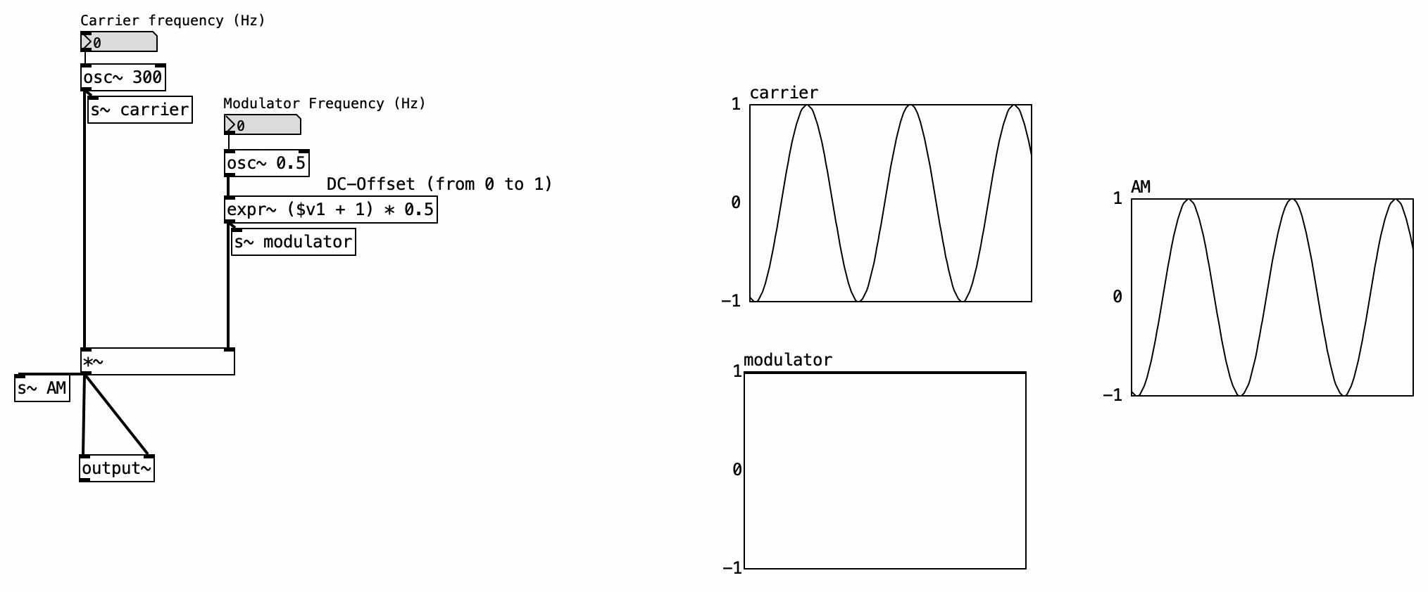
In the example provided, both the carrier and modulator are sine wave oscillators. This is what we call “classic” AM, where the modulator signal includes a DC offset, making it unipolar, ranging only from 0 to 1. This unipolarity ensures that the carrier’s amplitude is scaled without ever becoming negative.
4.4.2 Ring Modulation (RM)
RM is a particular form of AM where both the carrier and modulator signals are bipolar, meaning they oscillate between -1 and 1 without any DC offset. In this configuration, there’s no functional distinction between carrier and modulator—both behave symmetrically.
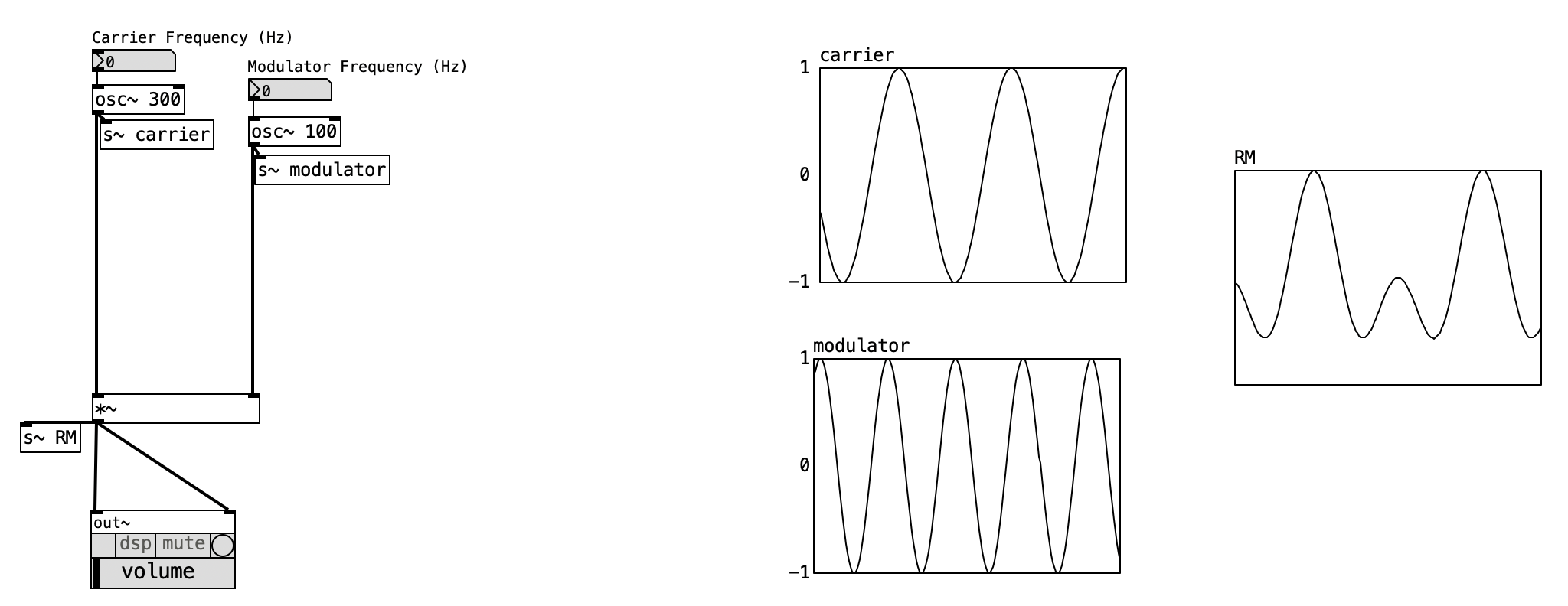
Nonetheless, in practical terms, the carrier is usually an audio signal such as a musical instrument, while the modulator remains a simple oscillator. A key technical detail is that when the modulator signal is negative, it inverts the polarity of the carrier signal—producing a unique and often metallic timbre.
4.4.3 DC Offset
AM schemes can involve various DC offset settings—not just limited to AM or RM. In our example, preset configurations for AM and RM are available, but one can also manually adjust peak levels and DC offset using sliders. Observe how, in the frequency spectrum of classic AM, we see two sidebands—above and below the carrier frequency—each at half the amplitude of the original carrier. These sidebands are spaced apart by the modulation frequency.
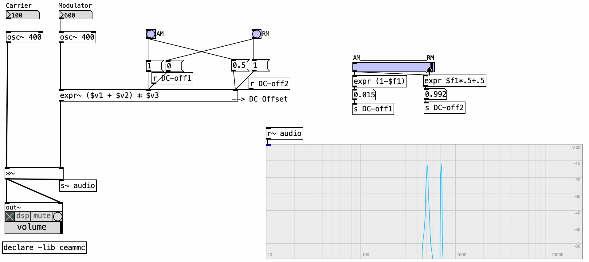
In contrast, RM removes the original carrier frequency entirely from the spectrum, leaving only the sidebands, which typically carry more energy than in AM.
By adjusting amplitude and DC offset with sliders, we can morph continuously between AM and RM modes, gaining nuanced control over the presence of the original frequency component and the energy distribution in the sidebands.
4.4.4 Audio Samples & Modulation
In this example, an audio sample replaces the oscillator as the carrier signal. This demonstrates how AM can function as an audio effect processor rather than just a synthesis technique. In fact, much of what we traditionally associate with synthesis techniques is often more accurately described as audio processing.
Conversely, many effects processors—such as filters—are integral to sound synthesis. The boundary between synthesis and processing is thus fluid and contextual.
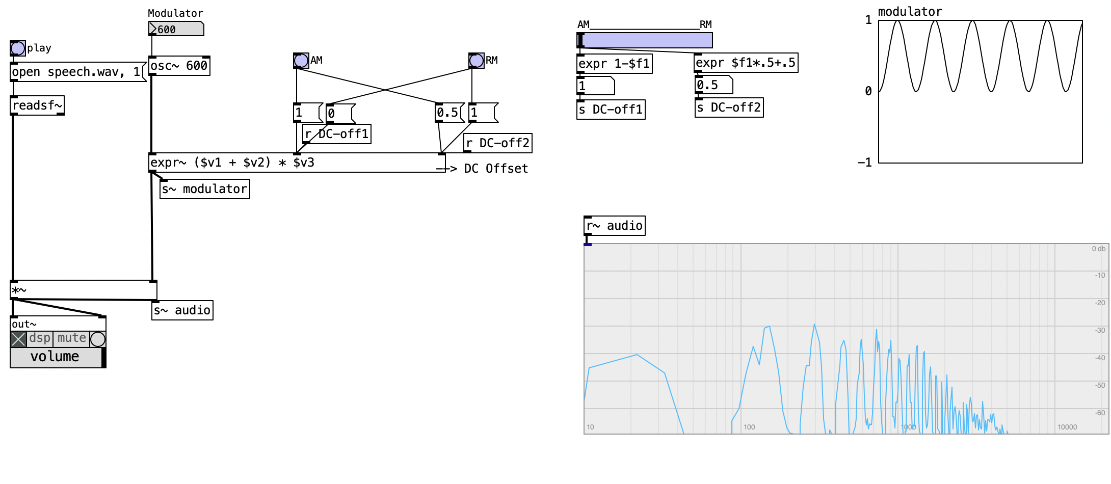
Try both the classic AM and RM examples. In both cases, sidebands are generated for each sine wave component within the carrier signal. AM retains the carrier’s original sine components, which coexist and interact with the generated sidebands. For this reason, AM is commonly used for tremolo effects (which we’ll examine later). On the other hand, RM removes the original sine components entirely, yielding a more sonically distinctive result.
4.4.5 Other Waveforms
Using more complex waveforms for the modulator signal leads to the creation of additional partials within any AM patch—including RM. Sine waves are typically favored as modulators since they offer clean and controlled results, especially when applying AM as an audio effect.
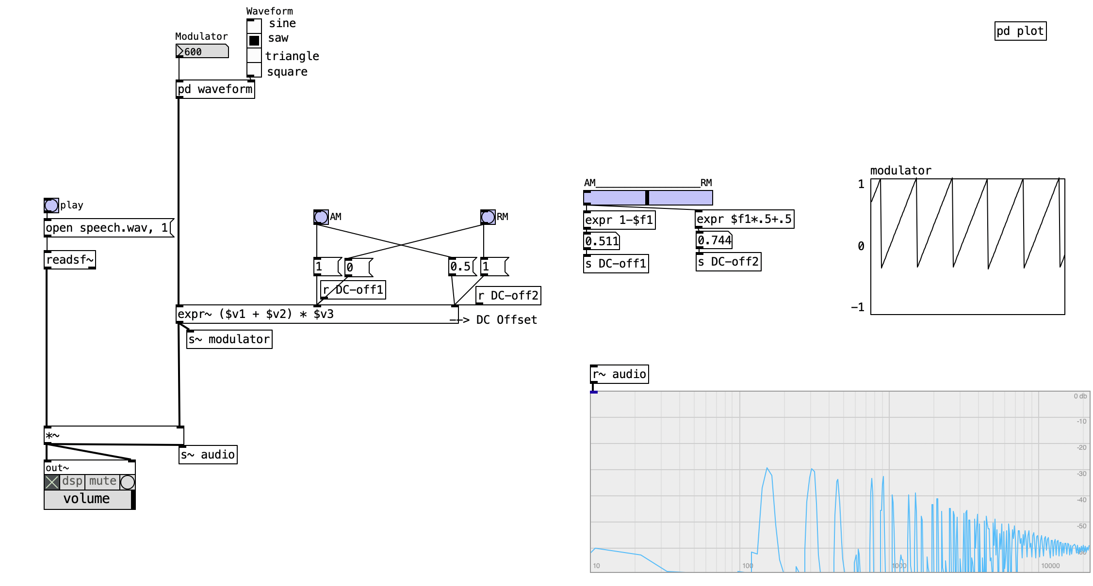
However, in synthesis contexts, more intricate and harmonically rich methods—such as frequency and phase modulation—offer more efficient and versatile approaches for generating complex timbres. We’ll explore these in the following sections.
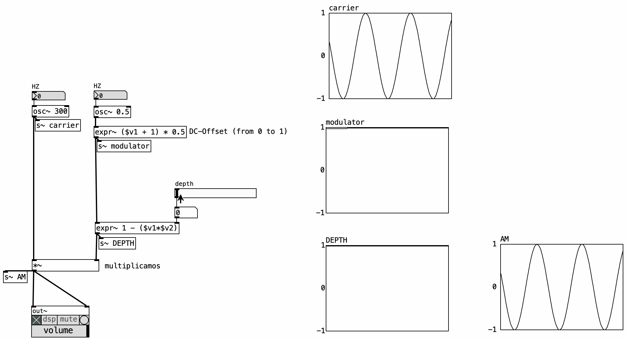
4.4.6 Tremolo
Tremolo is essentially AM using a low-frequency modulator (or a Low Frequency Oscilator - LFO). The key addition is a depth parameter, ranging from 0 to 1, which determines the modulation intensity. At 0, no modulation occurs (dry signal), while a depth of 1 results in full tremolo, where the carrier’s amplitude is modulated across its full range.
4.5 Frequency Modulation (FM)
In general terms, to modulate a signal means to alter it in some way. In the context of this course, however, we refer specifically to using a modulating signal to control a parameter—such as amplitude, as previously discussed. We now turn to the basic structure of frequency modulation (FM), where an oscillator acts as the modulator.
The signal being modulated is called the carrier; in the case of FM, it is also referred to as the carrier frequency. In contrast, we have the modulating frequency, which corresponds to the frequency of the modulating oscillator. The depth of frequency variation is determined by the amplitude of the modulator and is commonly referred to as the modulation index. The modulation process itself is straightforward: we add the modulating signal to the frequency input of the carrier oscillator.
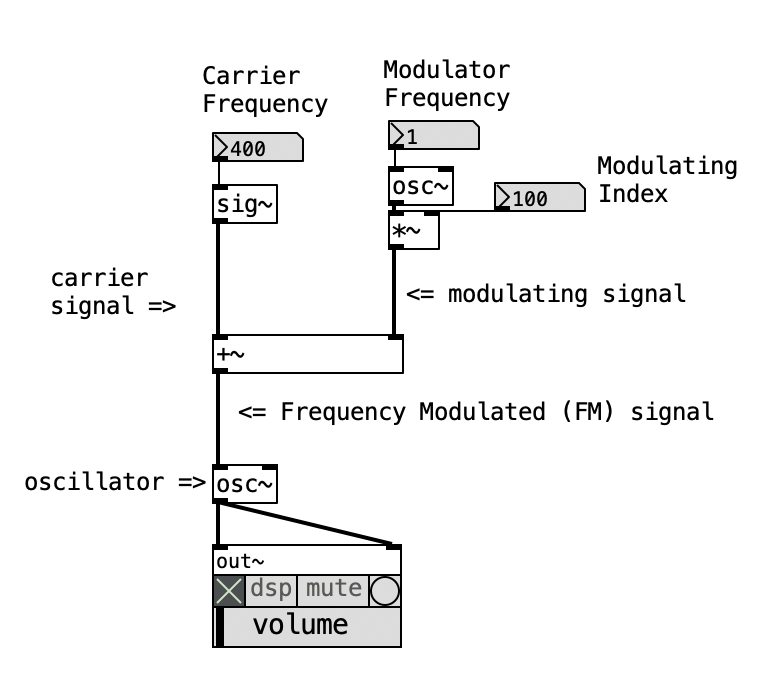
By default, we have a carrier frequency of 400 Hz, a low modulation frequency of 1 Hz, and a modulation index of 100. This means the modulating signal oscillates between -100 and +100 Hz, causing the carrier frequency to vary between 300 and 500 Hz. Note that when the modulation frequency is low, the result is a vibrato-like effect.
4.5.1 FM Simple
We apply the same structure as before. Besides a vibrato example, this section includes fully developed FM examples. As with amplitude modulation, FM produces sidebands spaced by intervals equal to the modulation frequency. However, FM can generate many more sidebands, potentially resulting in a much richer spectrum.
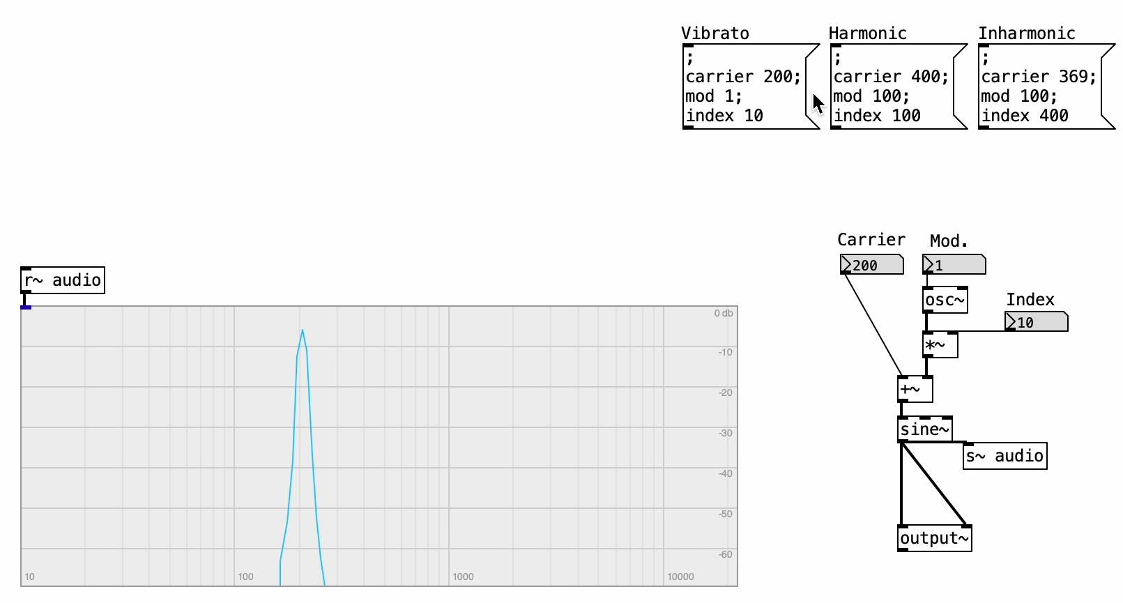
The higher the modulation index, the greater the number of resulting partials—enabling the creation of dense and complex waveforms. When the carrier and modulator frequencies share a simple harmonic ratio, the resulting waveform is harmonic. Otherwise, it tends to be inharmonic.
4.5.2 Other Waveforms
In this patch, we experiment with different oscillator combinations. Waveforms are arranged according to spectral complexity—from simple sine waves to rich sawtooth waves (the only waveform here containing both even and odd harmonics). The more complex the waveform used, the more intricate (and unpredectible) the FM result becomes.
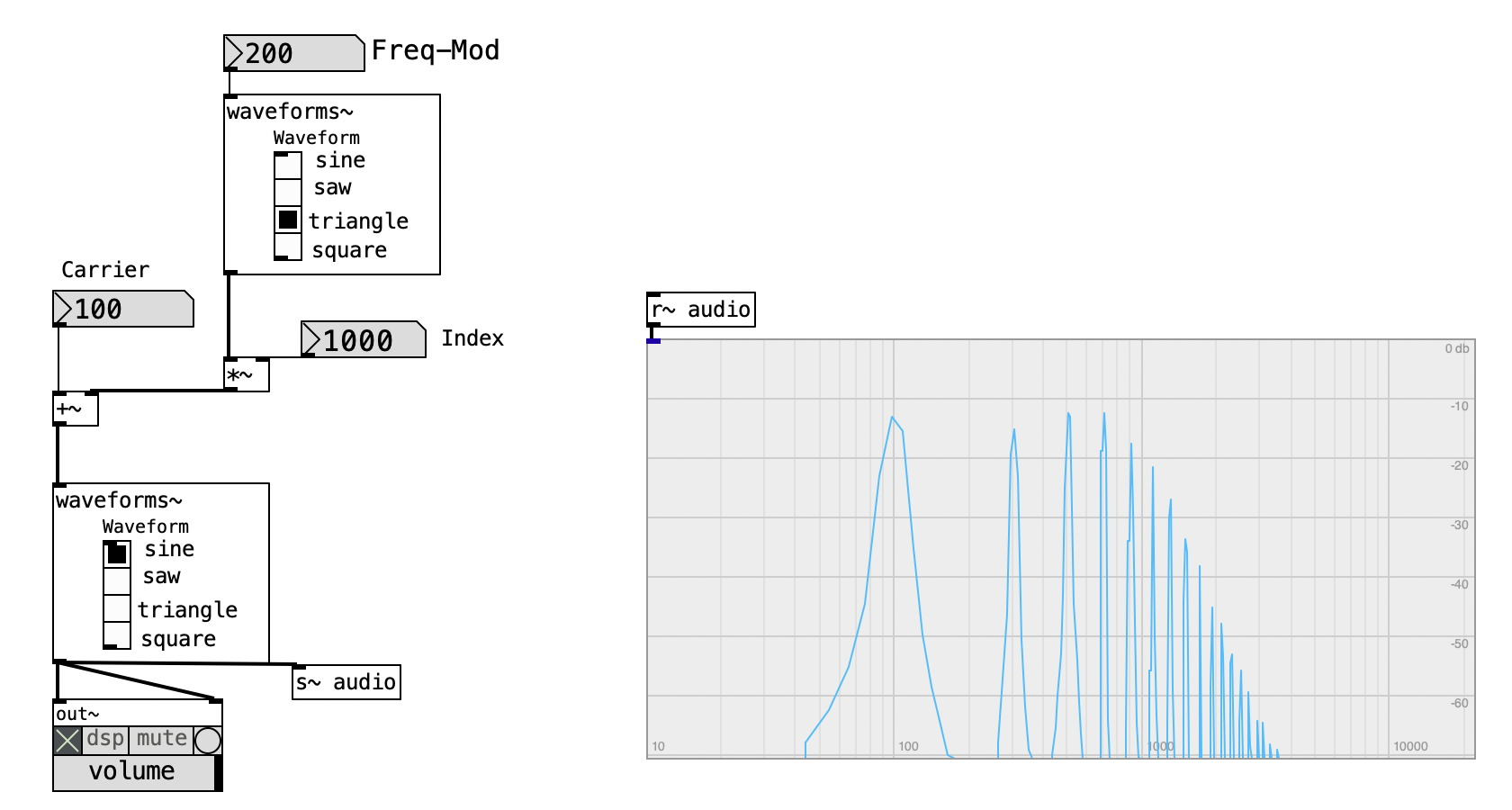
On the modulator side, the waveforms are idealized and band-unlimited—perfect in theory. However, the frequency-modulated oscillator has a limited bandwidth, which imposes practical constraints on the resulting spectrum.
4.5.3 Exponential Frequency
We can also use exponential pitch values (such as MIDI note numbers) instead of linear frequency input. The key difference here is that frequency deviation—the modulation index—is now expressed in semitones, not Hertz. This shift affects the entire modulation behavior.
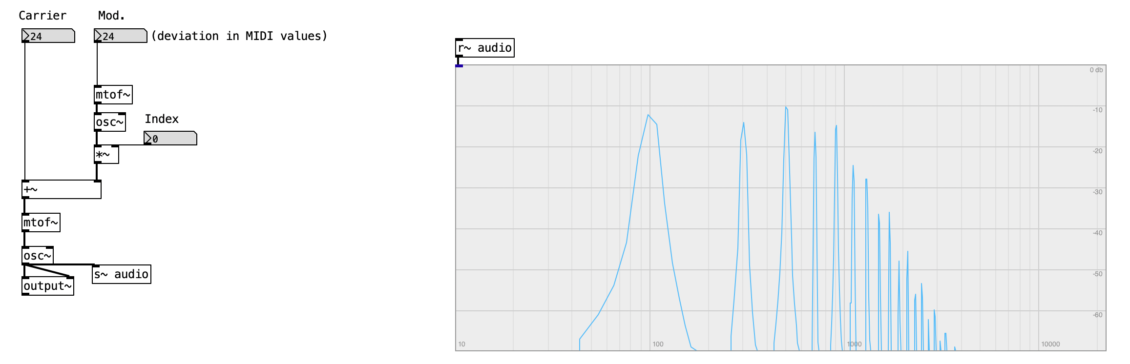
As a result, the output waveform becomes asymmetrical and significantly different in character. The main change in the patch is the use of [mtof~] to convert MIDI pitch to frequency in Hz.
4.5.4 Ratio
It is common practice to define the modulating frequency as a ratio of the carrier frequency. This allows us to work with a single frequency input while maintaining a consistent sonic character across different pitches.
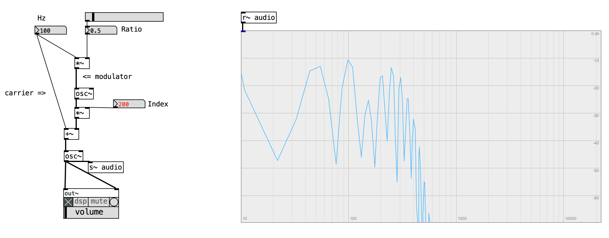
This approach preserves the relationship between the carrier and modulator frequencies, which is crucial since this ratio determines how the additional spectral components—partials—are distributed. Harmonic ratios (such as 0.5 or 2) yield harmonic results, while non-integer ratios lead to inharmonic spectra.
4.6 Subtractive Synthesis
Subtractive synthesis is frequently—and mistakenly—viewed as synonymous with analog synthesis. While there are many methods of sound synthesis, subtractive synthesis remains the most prevalent in commercial analog synthesizers. Often presented through user interfaces brimming with knobs and switches, it can appear overwhelming to newcomers. However, its intuitive one-to-one mapping between physical controls and sound parameters makes it especially suitable for educational contexts. Furthermore, it provides a useful entry point for exploring core acoustic principles and models of sound production.
4.6.1 Conceptual Model: Source and Modifier
At the heart of subtractive synthesis lies a conceptual framework: the separation of sound production into three functional components: 1. source, 2. modifier, and 3. controller.
This framework mirrors the structure of many acoustic instruments, most clearly in wind instruments. Take, for example, the clarinet: its vibrating reed acts as the source, while the resonant body functions as a modifier. The reed alone produces a sharp, buzzing tone; the body of the clarinet, essentially a cylindrical tube, shapes this tone through its resonant properties, which are determined by physical dimensions like length and bore diameter. Together, they produce the rich timbral identity of the clarinet.
This model, while illustrative, is not universally applicable. Consider the guitar: its sound emerges from the interplay between the plucked string (source) and the resonant body (modifier). Yet unlike the clarinet, the source and modifier in the guitar are tightly coupled and difficult to separate experimentally. The string cannot be plucked in isolation, nor can the body’s resonant characteristics be accurately studied without the tensioned string.
Despite such limitations, the core idea—modifying a source signal to shape its timbre—is both intuitive and powerful. It underpins most approaches to sound synthesis and provides a compelling framework for creative exploration. In a subtractive synthesis context, this source-modifier model is streamlined: the sound source is designed to contain rich harmonic content, and the modifier (typically a filter) removes selected frequency components to shape the sound. The process is thus subtractive in nature—the unwanted frequencies are “subtracted” from the original signal.
4.6.2 Sound Sources
The primary sound sources in analog subtractive synthesizers are waveform generators and noise sources. As mentioned, common waveforms include sawtooth, square, pulse, sine, and triangle waves—each chosen for their mathematical simplicity and electronic feasibility. These shapes carry predictable harmonic content: for instance, sawtooth waves contain both even and odd harmonics, while square waves contain only odd harmonics.
Random waveforms, typically perceived as noise, include all frequencies and are often used to generate percussive or atmospheric textures. The devices that produce these waveforms—oscillators—are descendants of function generators. In subtractive synthesis, these oscillators produce continuous signals, with frequency typically controlled by voltage. These signals serve as raw material for further shaping via modifiers.
4.6.3 Filters
Filters play a central role in subtractive synthesis. At their core, filters are amplifiers whose gain varies with frequency. In most synthesizer contexts, filters are designed such that their maximum gain is one; thus, it’s more accurate to say that they attenuate different frequency components to varying degrees. When a filter’s parameters can be controlled via voltage, it becomes a Voltage-Controlled Filter (VCF). VCFs are essential modifiers because they allow dynamic control over a signal’s spectral content, significantly influencing the resulting timbre.
4.6.4 Classification of Filters
Filters are typically categorized by their frequency response—how they affect different parts of the frequency spectrum. There are four main types:
Low-pass filters (LPF) allow frequencies below a cutoff point to pass and attenuate higher frequencies. The cutoff frequency is defined as the point at which the signal is attenuated by 3 dB (the “half-power” point). The slope of attenuation is determined by the filter’s design: a one-pole filter attenuates at 6 dB per octave, a two-pole at 12 dB, and so on. Filters with steeper slopes, such as four-pole filters (24 dB/octave), tend to sound more “synthetic” and dramatically alter timbre.
High-pass filters (HPF) do the reverse, removing low frequencies and allowing higher frequencies to pass. This has the effect of “thinning” the sound by removing its fundamental or lower harmonics. HPFs are often used in combination with LPFs to further sculpt the timbre, especially when the goal is to mimic instruments with weak or missing fundamentals.
Band-pass filters (BPF) permit only a specified range of frequencies to pass. This is useful for emphasizing particular harmonic regions or simulating acoustic resonances. A BPF can be implemented by combining an HPF and an LPF in series. The central frequency of the pass-band is its resonant peak, and the width of the pass-band is termed the bandwidth.
Notch filters, or band-reject filters, remove a narrow band of frequencies, allowing all others to pass. These are useful for eliminating unwanted harmonics or resonant peaks, especially in applications such as feedback suppression or timbral correction.
Each filter type can be modulated dynamically, allowing timbral variation over time. For instance, sweeping the cutoff frequency of an LPF from high to low removes successive harmonics, gradually “closing” the filter and making the sound darker and more subdued.
The subtractive model—source rich in harmonics, modified via filtering—forms the foundational paradigm for analog synthesis. While conceptually straightforward, it allows for a wide array of sonic possibilities. By carefully selecting waveforms, modulating filter parameters, and controlling amplitude envelopes, one can sculpt intricate, evolving timbres.
This approach, despite its age, remains vital in modern synthesis. Its clarity, intuitiveness, and direct mapping between sound components and control structures make it an enduring framework for both education and creative practice. Whether one is emulating acoustic instruments or crafting entirely synthetic textures, subtractive synthesis offers a practical and powerful toolset for sonic exploration.
4.6.5 Filters in Pd
As mentioned, a filter is any process that modifies an incoming sound. From an acoustic perspective, filters are omnipresent: the reverberant characteristics of a room act as filters, as do the resonant bodies of musical instruments. Even the human vocal tract can be considered a natural filter. In our context, however, we define filters more narrowly: as signal processing modules—such as equalizers—that selectively amplify or attenuate specific frequency components of a sound.
The most common representation of how a filter affects sound is its frequency response. This is typically displayed as a graph where the horizontal axis represents frequency (in kilohertz), and the vertical axis shows amplitude (in decibels, dB). Positive values (above 0 dB) indicate frequencies that are being boosted, while negative values (below 0 dB) show those that are attenuated. In addition to frequency response, filters also affect the phase of the signal, which we refer to as phase response—representing the phase shift introduced as a function of frequency.
4.6.6 Low-Pass Filtering
The object lop~ in Pd (short for “low-pass”) implements a basic low-pass filter. This filter allows frequencies below a certain threshold, called the cutoff or roll-off frequency, to pass through while progressively attenuating higher frequencies. This transition is not abrupt: the filtering effect begins at 0 Hz and gradually increases, resulting in a -3 dB drop at the cutoff point. Beyond this, the attenuation rate is approximately 6 dB per octave.
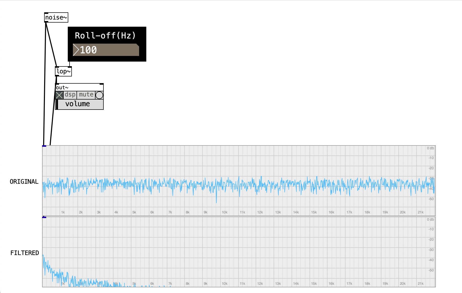
This filter is useful not only in audio synthesis but also in signal smoothing applications—such as envelope followers or data processing from physical sensors. At high cutoff frequencies (above ~5 kHz), the filter’s response deviates slightly from this ideal behavior.
4.6.7 High-Pass Filtering
A high-pass filter, such as hip~ in Pd, performs the inverse operation of a low-pass: it permits frequencies above a defined cutoff point and attenuates those below it. Interestingly, a high-pass effect can also be derived by subtracting the output of a low-pass filter from the original signal. While hip~ is often employed to remove DC offsets, it too has a 6 dB per octave slope and exhibits some gain anomalies at higher cutoff values.
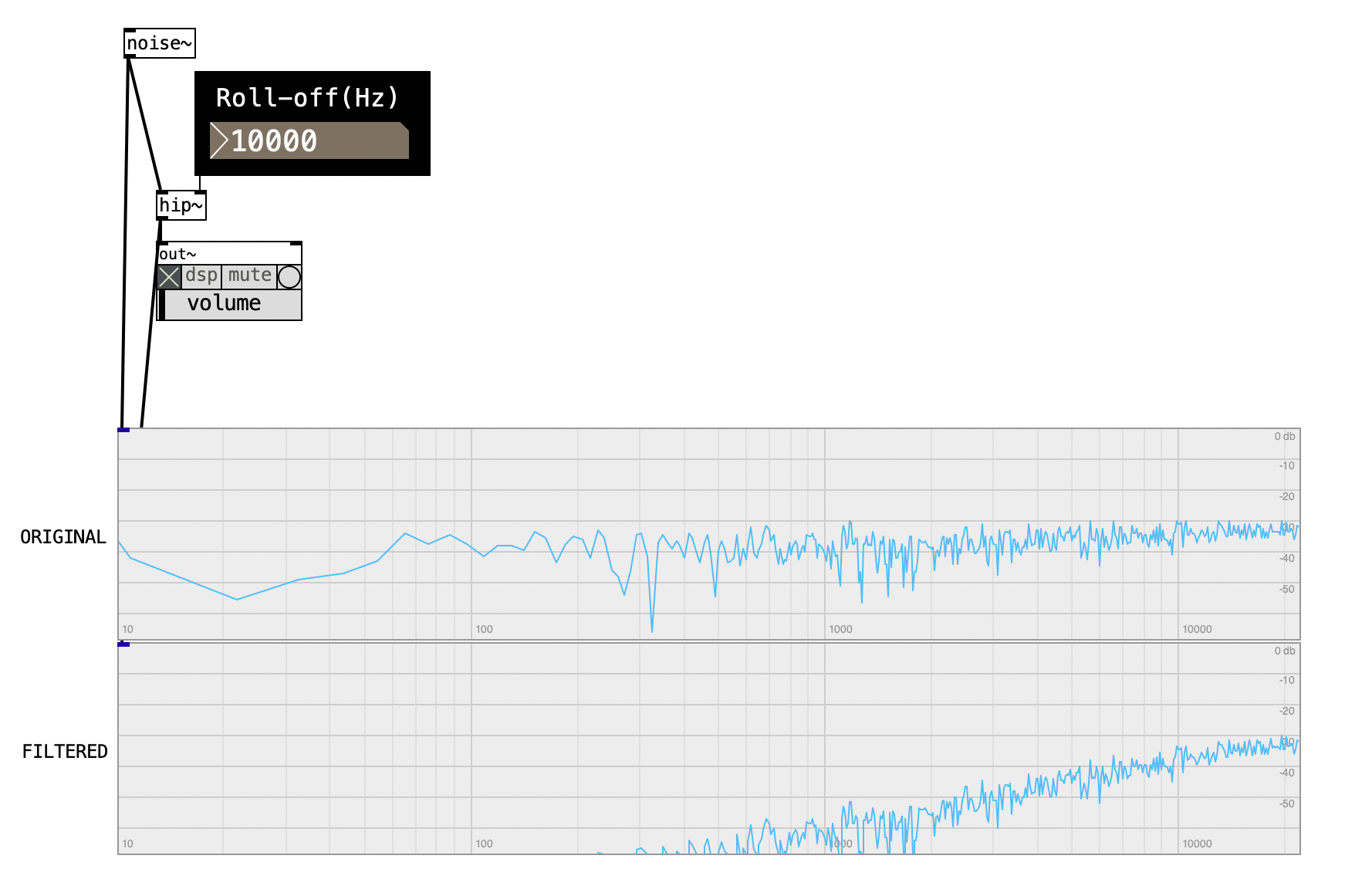
4.6.8 Resonant Filters
A resonant filter emphasizes a specific frequency band over others. A typical example is the band-pass filter, which allows only a defined range of frequencies to pass while attenuating those outside the band. The center frequency of this band is commonly denoted as ( f_0 ), with ( f_1 ) and ( f_2 ) marking the -3 dB points below and above it, respectively.
The bandwidth of the filter is defined as the difference between these two frequencies:
\[ \text{Bandwidth} = f_2 - f_1 \]
The musical interval between ( f_1 ) and ( f_2 ) can also be used to conceptualize the resonance more musically, especially when represented on a logarithmic scale like MIDI pitch.
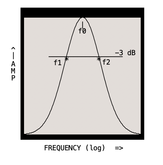
4.6.9 The Q Factor
The sharpness or “quality” of a filter’s resonance is quantified by the Q factor, which is calculated as:
\[ Q = \frac{f_0}{f_2 - f_1} \]
A higher Q value indicates a narrower and more pronounced resonance, while a lower Q results in a broader and more subtle response. In essence, Q and bandwidth are inverse measures of the same characteristic.
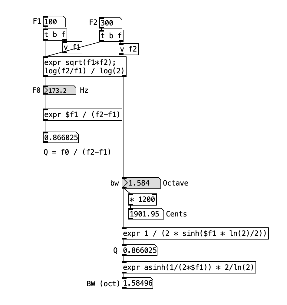
4.6.10 Band-Pass Filters
The bp~ object in Pd provides a straightforward implementation of a band-pass filter, accepting center frequency and Q as inputs. It is computationally efficient and practical, though it tends to attenuate frequencies above the center more than those below, thus producing an asymmetrical response. With a Q of 1, bp~ approximates the behavior of a lop~ filter. As with other vanilla filters, its frequency response changes noticeably at higher frequencies.
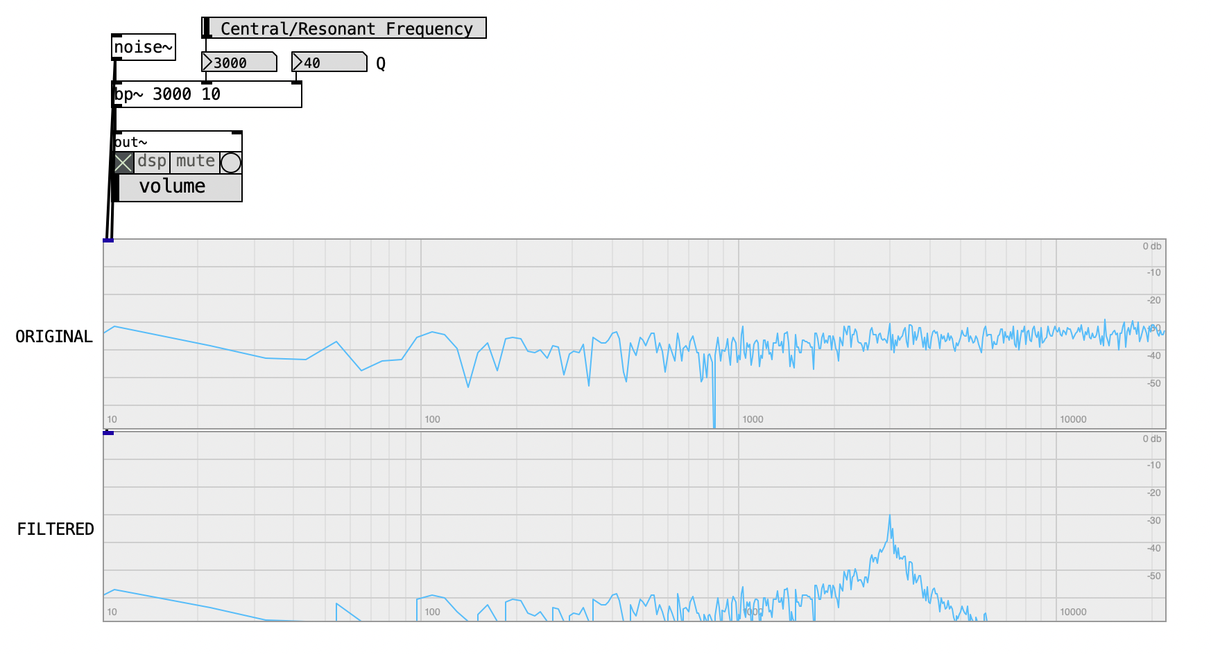
4.6.11 Voltage-Controlled Filters
The vcf~ object (short for “voltage-controlled filter”) is another band-pass filter in the vanilla distribution, notable for its ability to accept audio-rate signals to modulate the center frequency—mimicking the behavior of analog synthesizers. While the Q parameter is controlled by control-rate data, the central frequency can be dynamically shaped by audio input.
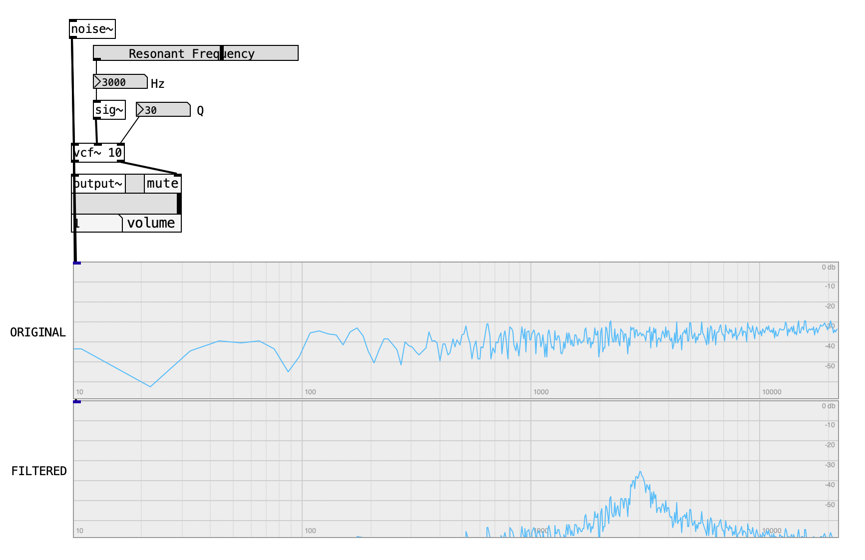
This object has two outputs: the right outlet approximates a bp~ filter’s frequency response, whereas the left outlet provides a complementary phase response. At low Q values, both outputs show a characteristically asymmetrical frequency curve, and deviations become more pronounced at higher frequencies (above ~7 kHz).
4.6.12 Emulating the Moog Filter
The bob~ object is a recent addition to Pd’s vanilla library, designed to model the iconic Moog filter created by Robert Moog. It allows both the cutoff frequency and Q to be modulated at audio rate, making it one of the most expressive and flexible filters in the system. Though officially described as a low-pass resonant filter, its architecture lends itself to a wide variety of applications. Users are encouraged to consult its help patch for in-depth understanding and examples.
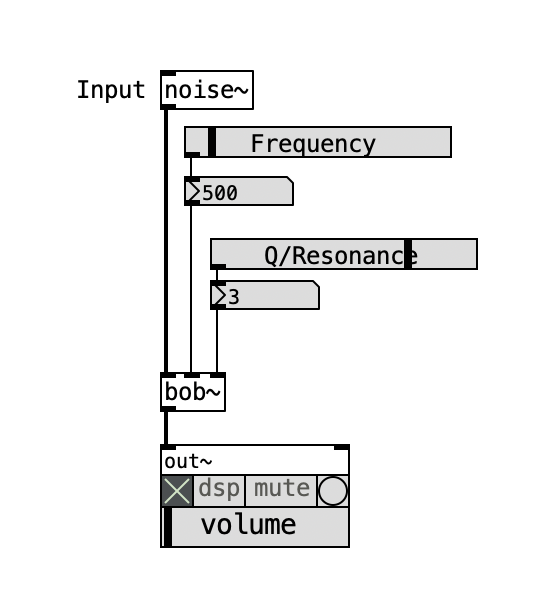
4.6.13 Biquad Filters
The biquad~ object is a versatile, coefficient-driven filter capable of implementing multiple filter types based on its settings. “Biquad” stands for “biquadratic,” reflecting its mathematical foundation in second-order polynomials. However, configuring biquad~ manually is a non-trivial task for most musicians or artists.
To simplify this process, the bicoeff object from the ELSE library allows users to generate coefficients for nine different filter types, based on Robert Bristow-Johnson’s “Cookbook formulae for audio EQ biquad filter coefficients”(Bristow-Johnson 2024). This GUI-based object visualizes the amplitude response in real time. The X-axis is logarithmic (typically in MIDI pitch), and the Y-axis represents gain in dB. Interactive controls allow users to modify frequency, bandwidth, and gain directly by clicking and dragging on the graph.
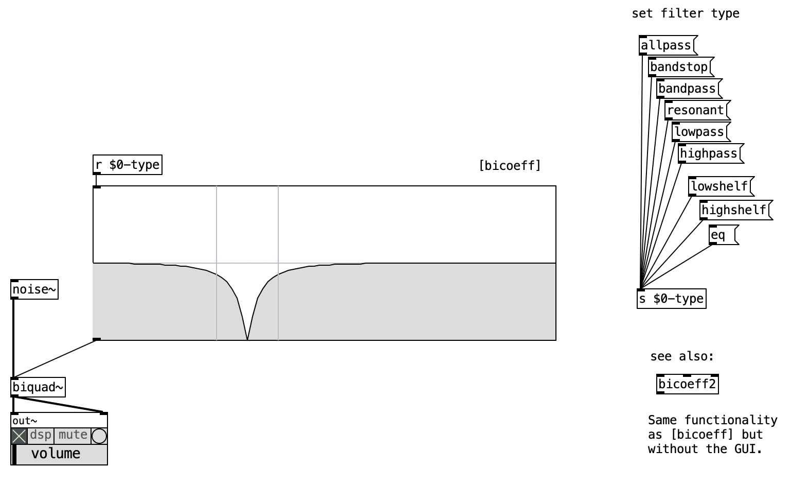
Together, these filtering tools illustrate the conceptual and practical range of subtractive and resonant filtering in sound synthesis. Whether you are shaping a simple tone, cleaning up sensor data, or building complex timbral transformations, understanding how filters operate is essential. They not only alter the spectral content of signals but also engage with broader perceptual dimensions—allowing composers, performers, and designers to sculpt sound with nuance and precision.
References
Bristow-Johnson, Robert. 2024. “Cookbook Formulae for Audio Equalizer Biquad Filter Coefficients.” https://webaudio.github.io/Audio-EQ-Cookbook/audio-eq-cookbook.html.
Helmholtz, Hermann. 1954. On the Sensations of Tone as a Physiological Basis for the Theory of Music. 2nd ed. New York: Dover Publications.
Lévi-Strauss, Claude. 1964. Le Cru Et Le Cuit. Vol. 1. Mythologiques. Paris: Plon.
Puckette, Miller. 2007. The Theory and Technique of Electronic Music. World Scientific Publishing. https://doi.org/10.1142/6277.
Sterne, Jonathan, and Tara Rodgers. 2011. “Poetics of Signal Processing.” Differences 22 (2-3): 31–53. https://doi.org/10.1215/10407391-1428834.
Théberge, Paul. 1997. Any Sound You Can Imagine: Making Music/Consuming Technology. Hanover & London: Wesleyan University Press.