graph TD
    A[electrocardiogram.txt] --> B[readtxt subpatch]
    B --> C[Array Sizing]
    A --> D[Array Loading]
    D --> E[tabread4~ Audio Reader]
    F[Phasor~ Oscillator] --> E
    E --> G[freeverb~ Reverb]
    G --> H[Audio Output]
    B --> I[Data Count Output]
5 Sonification
In this chapter, we will explore the concept of sonification, its applications, and how it can be implemented using Pd. We will also discuss the importance of understanding data types and classifications in the context of sonification.
5.1 Introduction
Imagine hearing the changes in global temperature over the past thousand years. What does a brainwave sound like? How can sound be used to enhance a pilot’s performance in the cockpit? These intriguing questions, among many others, fall within the realm of auditory display and sonification.
Researchers in Auditory Display explore how the human auditory system can serve as a primary interface channel for communicating and conveying information. The goal of auditory display is to foster a deeper understanding or appreciation of the patterns and structures embedded in data beyond what is visible on the screen. Auditory display encompasses all aspects of human-computer interaction systems, including the hardware setup (speakers or headphones), modes of interaction with the display system, and any technical solutions for data collection, processing, and computation needed to generate sound in response to data.
In contrast, sonification is a core technique within auditory display: the process of rendering sound from data and interactions. Unlike voice interfaces or artistic soundscapes, auditory displays have gained increasing attention in recent years and are becoming a standard method alongside visualization for presenting data across diverse contexts. The international research effort to understand every aspect of auditory display began with the founding of the International Community for Auditory Display (ICAD) in 1992. It is fascinating to observe how sonification and auditory display techniques have evolved in the relatively short time since their formal definition, with development accelerating steadily since 2011.
Auditory display and sonification are now employed across a wide range of fields. Applications include chaos theory, biomedicine, interfaces for visually impaired users, data mining, seismology, desktop and mobile computing interaction, among many others. Equally diverse is the set of research disciplines required for successful sonification: physics, acoustics, psychoacoustics, perceptual research, sound engineering, and computer science form the core technical foundations. However, psychology, musicology, cognitive science, linguistics, pedagogy, social sciences, and philosophy are also essential for a comprehensive, multifaceted understanding of the description, technical implementation, usage, training, comprehension, acceptance, evaluation, and ergonomics of auditory displays and sonification in particular.
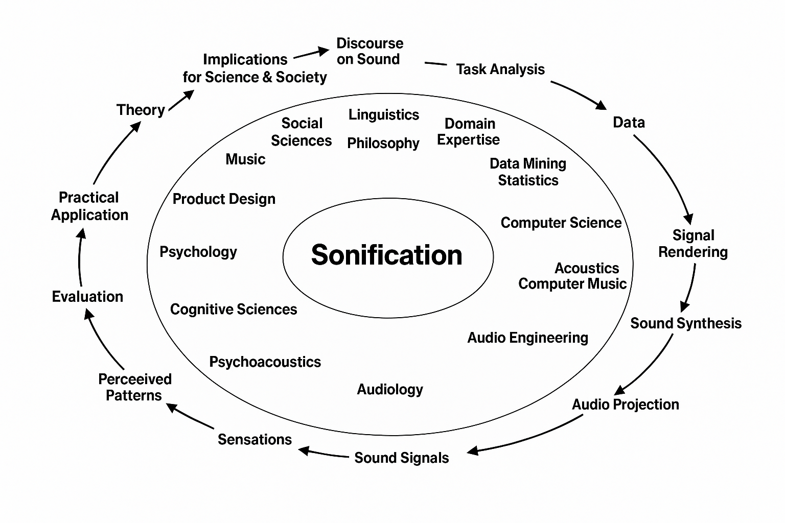
It is clear that in such an interdisciplinary field, a narrow focus on any single discipline risks “seeing the trees but missing the forest.” As with all interdisciplinary research efforts, auditory display and sonification face significant challenges, ranging from differing theoretical orientations across fields to even the very vocabulary used to describe our work.
Interdisciplinary dialogue is crucial to advancing auditory display and sonification. However, the field must overcome the challenge of developing and employing a shared language that integrates many divergent disciplinary ways of speaking, thinking, and approaching problems. On the other hand, this very challenge often unlocks great creative potential and new ideas, as these varied perspectives can spark innovation and fresh insights.
5.2 Data Types
In the realm of digital data, understanding the nature and classification of data types is essential for their effective processing, storage, and analysis. The table above presents a detailed taxonomy of data types broadly categorized into Static and Stream / Realtime data, further subdivided into various subtypes. This section will unpack these classifications, elaborating on their characteristics, common formats, and sources.
5.2.1 Static Data
Static data refers to data that is stored and remains unchanged until explicitly modified. It is typically collected, stored, and then analyzed or processed offline or asynchronously. This type of data is fundamental in many computational tasks, including machine learning, data mining, and archival storage.
5.2.1.1 Structured Data
Structured data is organized in a predefined manner, typically conforming to a schema or model that allows easy querying and manipulation.
Examples:
- Datasets (CSV, XLS): Tabular data with rows and columns, where each column has a defined datatype (e.g., numeric, string, datetime).
- Fields: The basic elements of structured data that have specific data types, such as integers, floating-point numbers, text strings, or timestamps.
- Classes: Labels used in supervised learning, often binary (two classes) or multiclass (multiple categories).
- Images: Digital images can be structured if stored with metadata or standardized file formats. Examples include compressed formats like JPG and uncompressed formats like BMP.
- MIDI Files: Musical Instrument Digital Interface files encode structured note and control information.
- Audio: Raw waveforms or extracted descriptors (e.g., Mel-frequency cepstral coefficients - MFCCs, Fourier transforms) represent audio signals in structured formats.
- Audio Formats: Common audio file formats such as MP3 (compressed), FLAC (lossless compressed), and WAV (uncompressed).
Sources: Data portals (e.g., Kaggle, UCI Machine Learning Repository), social media platforms like Instagram, Reddit, Flickr (for images), and audio repositories.
5.2.1.2 Semi-structured Data
Semi-structured data does not conform to a rigid schema like structured data but still contains tags or markers to separate semantic elements.
Examples:
- Markup Languages: HTML, XML, JSON, and YAML files are examples of semi-structured data because they contain hierarchical tags and attributes describing the data, but the content may be variable.
Sources: Web content, APIs that deliver data in JSON or XML formats.
5.2.1.3 Unstructured Data
Unstructured data lacks a predefined data model or schema. It is the most common form of data generated and can be more challenging to analyze without preprocessing.
Examples:
- Texts: Documents, emails, articles, or social media posts are typical unstructured data examples.
Sources: Document collections, text corpora, email archives.
5.2.2 Stream / Realtime Data
Stream or realtime data refers to continuous data generated in real-time, often requiring immediate or near-immediate processing. These data types are crucial in applications like live monitoring, interactive systems, and real-time analytics.
Examples:
- Audio Streams: Continuous audio feeds such as online radio broadcasts.
- Video Streams: Live video feeds from CCTV cameras or autonomous vehicles.
- Sensor Data: Real-time telemetry or environmental data from IoT devices, Arduino boards, or embedded systems.
- Live MIDI: Streaming musical performance data, used in live concerts or interactive installations.
- OSC (Open Sound Control): A protocol used for networking sound synthesizers, computers, and other multimedia devices, enabling real-time control.
Sources: Online radio platforms, surveillance systems, smart vehicles, embedded IoT devices, live music performance setups.
5.2.3 Data Classification
The classification of data into static and stream/realtime reflects fundamentally different operational paradigms in digital systems. Static data often allows batch processing, archival, and complex analysis without stringent timing constraints. In contrast, stream data demands continuous, low-latency processing to support live feedback, monitoring, or interaction.
The structured / semi-structured / unstructured distinction highlights the complexity of dealing with data formats:
- Structured data is well-suited for traditional databases and straightforward analysis.
- Semi-structured data requires flexible parsers and understanding of nested or tagged data.
- Unstructured data often necessitates advanced techniques such as natural language processing or computer vision for meaningful extraction.
Understanding these data types and their sources is critical when designing systems for data ingestion, storage, processing, and analysis — especially in fields such as machine learning, multimedia processing, and IoT applications.
| Type | Subtype | Examples | Sources |
|---|---|---|---|
| Static | Structured Semi-structured Unstructured |
|
|
| Stream / Realtime | — |
|
|
5.2.3.1 References
Gantz, J., & Reinsel, D. (2012). The Digital Universe in 2020: Big Data, Bigger Digital Shadows, and Biggest Growth in the Far East. IDC iView.
Marr, B. (2016). Big Data in Practice: How 45 Successful Companies Used Big Data Analytics to Deliver Extraordinary Results. Wiley.
5.3 Sonification as a Creative Framework
Sonification, traditionally defined as the systematic, objective, and reproducible translation of data into sound, finds itself at a dynamic intersection between scientific inquiry and creative expression. While often framed within the methodological rigor of data representation, its deeper potential lies equally in its artistic embodiment—an expressive convergence of logic, perception, and auditory imagination. This duality is vital when considering the use of software in the development of creative code practices for sonification. In its essence, sonification provides a means to explore and interpret data temporally. It transforms static information into dynamic sonic experiences, revealing patterns not just to the analytical mind but to the aesthetic ear. As Gresham-Lancaster (Gresham-Lancaster 2012) argues, the field must extend beyond scientific formalism to embrace a broader spectrum of cultural and musical meaning.
A foundational concept introduced by Gresham-Lancaster is the distinction between first-order and second-order sonification. First-order sonification typically involves straightforward mapping of data points to sound parameters—e.g., a numerical value controlling oscillator frequency or filter cutoff. This direct translation preserves the integrity of the data but may lack emotional resonance or contextual clarity for listeners unfamiliar with the dataset or mappings. Second-order sonification introduces a higher level of abstraction. Here, data is not merely converted to sound but is used to control compositional structures such as rhythm, harmony, timbre, and formal development. This could manifest through software designs that incorporate statistical analysis of datasets to determine musical motifs or drive stochastic processes that evolve over time. By embedding data within culturally familiar or stylistically resonant frameworks—be it ambient textures, rhythmic patterns, or harmonic progressions allows the sonification to become more legible and emotionally impactful.
A key insight is that listeners inevitably interpret sound within a cultural and stylistic frame. Whether intentional or not, sonification software maps data to sonic outputs will be perceived through the lens of genre conventions—ambient, noise, glitch, minimalism, etc. This reinforces the necessity for designers of sonification systems to consciously engage with aesthetic decisions. Rather than viewing these as distractions from scientific rigor, they should be recognized as essential design variables that determine how well the sonification communicates. For instance, layering the sonified stream within an evolving drone texture or embedding it in rhythmic pulses tied to diurnal cycles may enhance the intelligibility of subtle shifts. These choices, while extramusical, profoundly affect the user’s ability to detect and interpret meaningful changes.
The expressive capacity of sonification technics invites an analogy with sculpture, as cited in Xenakis’ conception of raw mathematical outputs as “virtual stones” to be artistically shaped. The creative coder similarly refines the raw outputs of data-driven patches, sculpting auditory forms through iterative experimentation, parameter tuning, and aesthetic discernment. This process reveals sonification not as a deterministic output of data, but as a collaboration between the structure of information and the intuition of the artist-programmer. Moreover, by incorporating techniques such as timbral mapping, adaptive filtering, and data-driven granular synthesis, it becomes a laboratory for crafting sonic experiences that honor both the source data and the listener’s perceptual world. This is particularly effective when the goal is to embed sonification within broader artistic or performative contexts—installations, interactive systems, or generative concerts—where expressivity and audience engagement are critical.
The evolution of sonification within the creative coding domain demands a reconceptualization of what constitutes success in sonification. Beyond reproducibility, the true measure lies in perceptual clarity, aesthetic engagement, and communicative power. As Gresham-Lancaster asserts, the inclusion of musical form, stylistic awareness, and cultural embedding are not luxuries, but necessities for sonification to become a widely adopted and meaningful practice Pd, with its flexibility, open-ended structure, and visual coding paradigm, provides an ideal environment to develop and test both first-order and second-order sonification systems. By embracing both scientific precision and artistic insight, Pd-based sonification becomes a model for interdisciplinary practice—where the auditory exploration of data is not just informative but transformative.
5.4 Data Sonification Artworks Database
The following links provides an overview of notable sonification artworks, highlighting their creators, data sources, and the unique approaches they employ to transform data into sound.
Data Sonification Archive - curated collection is part of a broader research endeavor in which data, sonification and design converge to explore the potential of sound in complementing other modes of representation and broadening the publics of data. With visualization still being one of the prominent forms of data transformation, we believe that sound can both enrich the experience of data and build new publics.
Sonification Art database by Samuel Van Ransbeeck - It contains now 256 projects, making it an interesting catalogue for sonification art. Besides adding new works, I also cleaned up some things.
5.5 Data Humanism: A Visual Manifesto of Giorgia Lupi
Data is now recognized as one of the foundational pillars of our economy, and the idea that the world is exponentially enriched with data every day has long ceased to be news.
Big Data is no longer a distant dystopian future; it is a commodity and an intrinsic, iconic feature of our present—alongside dollars, concrete, automobiles, and Helvetica. The ways we relate to data are evolving faster than we realize, and our minds and bodies are naturally adapting to this new hybrid reality built from physical and informational structures. Visual design, with its unique power to reach deep into our subconscious instantly—bypassing language—and its inherent ability to convey vast amounts of structured and unstructured information across cultures, will play an even more central role in this quiet yet inevitable revolution.
Pioneers of data visualization like William Playfair, John Snow, Florence Nightingale, and Charles Joseph Minard were the first to harness and codify this potential in the 18th and 19th centuries. Modern advocates such as Edward Tufte, Ben Shneiderman, Jeffrey Heer, and Alberto Cairo have been instrumental in the field’s renaissance over the past twenty years, supporting the transition of these principles into the world of Big Data.
Thanks to this renewed interest, an initial wave of data visualization swept across the web, reaching a wider audience beyond the academic circles where it had previously been confined. Unfortunately, this wave was often ridden superficially—used as a linguistic shortcut to cope with the overwhelming nature of Big Data.
“Cool” infographics promised a key to mastering this untamable complexity. When they inevitably failed to deliver on this overly optimistic expectation, we were left with gigabytes of illegible 3D pie charts and cheap, translucent user interfaces cluttered with widgets that even Tony Stark or John Anderton from Minority Report would struggle to understand.
In reality, visual design is often applied to data merely as a cosmetic gloss over serious and complicated problems—an attempt to make them appear simpler than they truly are. What made cheap marketing infographics so popular is perhaps their greatest contradiction: the false claim that a few pictograms and large numbers inherently have the power to “simplify complexity.” The phenomena that govern our world are, by definition, complex, multifaceted, and often difficult to grasp. So why would anyone want to dumb them down when making critical decisions or delivering important messages?
Yet, not all is bleak in this sudden craze for data visualization. We are becoming increasingly aware that there remains a considerable gap between the real potential hidden within vast datasets and the superficial images we typically use to represent them. More importantly, we now recognize that the first wave succeeded in familiarizing a broader audience with new visual languages and tools.
Having moved past what we might call the peak of infographics, we are left with a general audience equipped with some of the necessary skills to welcome a second wave of more meaningful, thoughtful visualization.
We are ready to question the impersonality of a purely technical approach to data and begin designing ways to connect numbers with what they truly represent: knowledge, behaviors, and people.
Certainly. Here’s a refined and academically styled rephrasing of the provided section, maintaining clarity, structure, and alignment with the tone of an academic book:
5.5.1 Data Humanism and Personal Data
Data Humanism is a perspective initially articulated by Giorgia Lupi (Lupi 2017), grounded in the belief that meaningful engagement with data necessitates attention to its underlying contexts and the inclusion of subjective perspectives throughout the processes of data collection, analysis, and representation—particularly when the data reflects human experience. Rather than reducing information to mere numbers or abstractions, Data Humanism emphasizes the value of personalized, context-rich, and narratively driven interpretations. It advocates for a relationship with data that is not only analytical but also emotional, aesthetic, and reflective (Canossa et al. 2022).
This orientation has gained considerable traction within the domains of personal informatics and personal visualization, which investigate how individual-centered representations—visual or tangible—can support self-awareness, reflective thinking, and behavior change. Within these fields, Data Humanism has informed two primary dimensions: data representation and the sensemaking process.
5.5.2 Data Representation
From the perspective of Data Humanism, effective data representation involves the creation of complex and personalized visual forms. “Complexity” here does not imply obfuscation, but rather a deliberate move beyond conventional charts and graphs, toward expressive visual metaphors capable of revealing unexpected connections and enriching the narrative potential of the data (Kim et al. 2019).
Personalization plays a crucial role in enabling individuals to define and structure data in accordance with their own conceptual frameworks, thus making the resulting representations more relevant and resonant. Moreover, contextual information—embedded at all stages of the data pipeline from collection to display—is essential for constructing coherent and situated personal narratives. This approach aligns with broader discourses in data visualization research that call for expressive and nuanced visual forms, capable of communicating layered meanings rather than merely delivering rapid information.
5.5.3 Sensemaking Process
Data Humanism also foregrounds the importance of deep, deliberate engagement in the interpretive act of making sense of data. As Lupi (Lupi 2017) observes, insight does not emerge from superficial scanning but from a sustained exploration of context and meaning. In this light, the process of data sensemaking is framed as investigative, interpretive, and relational, acknowledging the imperfection and approximation that are often intrinsic to human data.
This approach encourages individuals to participate actively in the shaping of their own data narratives—through exploration, translation, and imaginative visualization—which in turn facilitates deeper personal connections and empathetic understanding of others. These practices resonate with the concept of slow technology (Hallnäs and Redström 2001), which posits that slower, more reflective interactions can enrich user experience, enabling more space for contemplation and insight. Here, “slowness” is not a limitation but a strategic feature, fostering sustained attention and interpretive depth.
Recent work in personal visualization has explored how Data Humanism can be applied in practice. One avenue involves sketch-based visualization tools, which leverage the intuitive, open-ended nature of drawing to support the creation of personalized visual representations. Another involves constructive visualizations: physical, often non-digital artifacts that users assemble and manipulate to give form to data. Additionally, digital platforms have been developed that enable the design of expressive visualizations capable of capturing qualitative aspects of personal context, broadening the expressive range of data visual design.
Overall, Data Humanism advocates for data representations that embrace subjectivity and slowness as virtues rather than limitations. It proposes that personal data is best understood not through abstract generalization, but through thoughtful, expressive, and often collaborative processes. In this book, we extend this line of inquiry by examining how Data Humanism principles can be integrated into collaborative design practices for personal visualization—exploring new ways to humanize, materialize, and narrativize the data that defines and reflects our lives.
5.6 Electrocardiogram Data
This Pd patch represents an approach to biomedical data sonification, transforming electrocardiogram (ECG) readings into audible waveforms. By treating physiological data as audio samples, the patch creates an intersection between medical diagnostics and sound synthesis, offering both artistic and analytical possibilities for exploring cardiac rhythms through auditory perception.
5.6.1 Patch Overview
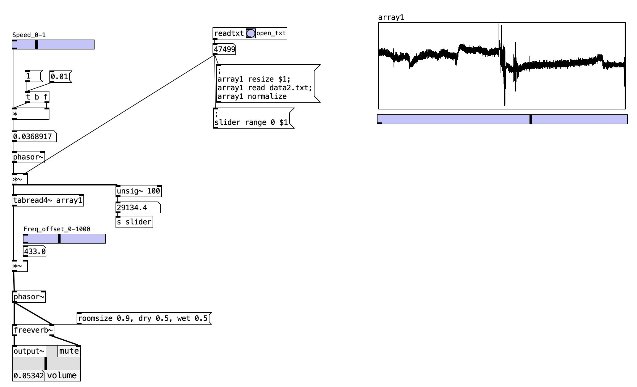
The electrocardiogram synthesis patch implements a data-to-audio pipeline that processes filtered ECG data stored in text format. The system loads cardiac waveform data into Pd arrays and uses audio synthesis techniques to render the biological signals as sound, enhanced with spatial reverberation effects.
The electrocardiogram.txt file contains preprocessed electrocardiogram (ECG) data representing cardiac electrical activity captured from a real patient or medical recording device.
5.6.1.1 Format Specification
- File Type: Plain text format (.txt)
- Data Points: 47,499 individual samples
- Value Range: Approximately 544 to 1,023
- Sampling Structure: One numerical value per line
- Data Type: Integer values representing digitized voltage measurements
5.6.1.2 Signal Properties
The ECG data exhibits characteristic patterns of cardiac electrical activity:
| Parameter | Value | Description |
|---|---|---|
| Baseline Level | ~830-850 | Resting electrical potential |
| Peak Amplitude | 1,023 | Maximum QRS complex values |
| Minimum Values | 544 | Deep S-wave deflections |
| Duration | Variable | Complete cardiac cycles with P-QRS-T patterns |
The high sample count (47,499 points) provides sufficient temporal resolution to capture multiple complete heartbeat cycles, enabling both detailed analysis of individual cardiac events and broader rhythm pattern recognition through auditory display techniques.
5.6.2 Data Flow
The readtxt subpatch serves as a preprocessing module that:
- Opens the electrocardiogram.txt file
- Counts the total number of data points
- Calculates appropriate array dimensions
- Provides sizing information for memory allocation
graph LR
    A[readtxt subpatch] --> B[Array Sizing]
    B --> C[Array Loading]
    C --> D[Audio Conversion]
The electrocardiogram sonification patch implements a data transformation pipeline that converts static physiological measurements into dynamic audio experiences. This process involves multiple interconnected stages of data handling, each contributing essential functionality to the overall system’s ability to render cardiac rhythms as meaningful sonic representations.
The initial phase of data flow centers on the comprehensive analysis and preparation of the source electrocardiogram dataset. The readtxt subpatch performs a preliminary scan of the electrocardiogram.txt file, systematically counting the total number of individual data points contained within the text document. This preprocessing step proves crucial for subsequent memory allocation decisions, as Pd requires explicit array dimensioning before data can be loaded into memory buffers. The subpatch communicates the determined data quantity to the main patch, enabling dynamic array sizing that accommodates datasets of varying lengths without requiring manual configuration adjustments. Following this analysis phase, the system initiates the actual data transfer process, where numerical values representing cardiac electrical activity are systematically loaded from the text file into Pd’s internal array structures. This loading operation transforms the static file-based data into a format suitable for real-time audio processing, creating a bridge between stored physiological measurements and live sonic synthesis.
The audio synthesis stage represents the core transformation where biological data becomes audible waveform. The phasor~ object generates a continuous ramp signal that serves as the fundamental timing mechanism for array traversal, essentially functioning as a playback head that moves through the stored ECG data at a controllable rate. This oscillator’s frequency parameter directly determines the speed at which the cardiac data is sonified, allowing for temporal scaling that can compress hours of ECG recordings into minutes of audio or extend brief cardiac events for detailed auditory analysis. The tabread4~ object performs the critical function of converting discrete array values into continuous audio signals through sophisticated interpolation algorithms. Rather than simply stepping through individual data points, which would produce harsh discontinuities and aliasing artifacts, the four-point interpolation scheme creates smooth transitions between adjacent values, resulting in audio output that maintains the natural flow characteristics of the original cardiac rhythms while remaining suitable for human auditory perception.
The final processing stage introduces spatial and timbral enhancements that transform the raw sonified data into aesthetically coherent audio suitable for both analytical and artistic applications. The freeverb~ object applies algorithmic reverberation that adds spatial depth and acoustic warmth. This reverberation processing serves multiple purposes: it masks potential digital artifacts from the sonification process, creates a more immersive listening environment that encourages extended auditory analysis, and provides timbral coherence that helps listeners focus on meaningful patterns rather than being distracted by the mechanical quality of direct data-to-audio conversion. The spatial processing also contributes to the patch’s potential for integration into larger sonic environments, where the ECG sonification might coexist with other audio elements in installations or performance contexts.
Throughout this entire data flow pathway, the system maintains precise temporal relationships between the original cardiac measurements and their auditory representations, ensuring that the sonification preserves the essential rhythmic and morphological characteristics that define cardiac health and pathology. This fidelity to source data temporal structure enables the sonification to serve legitimate diagnostic and educational purposes while simultaneously opening creative possibilities for artistic exploration of physiological processes.
graph LR
    A[Data Size] --> B[Array Efficiency]
    B --> C[Playback Smoothness]
    C --> D[Audio Quality]
The patch maintains signal integrity through:
- 4-point interpolation for anti-aliasing
- Configurable playback rates for temporal scaling
- Reverb processing for spatial contextualization
This electrocardiogram synthesis patch demonstrates Pd’s versatility in scientific data visualization through sound, creating meaningful auditory representations of biological processes while maintaining the temporal and amplitude characteristics essential for medical interpretation.
5.6.3 Key Objects and Their Roles
| Object | Function | Parameters |
|---|---|---|
readtxt |
Subpatch for file analysis | Counts data points in text file |
textfile |
File reading mechanism | Loads ECG data from external source |
table/array |
Data storage buffer | Holds ECG samples for playback |
phasor~ |
Playback control oscillator | Sweeps through array data |
tabread4~ |
Audio sample interpolator | Reads array as continuous audio |
freeverb~ |
Spatial audio processor | Adds reverberation to output |
5.7 ECG-Controlled Step Sequencer
This patch demonstrates an innovative approach to data-driven rhythm generation, where electrocardiogram readings function as temporal control signals for a step sequencer. By interpreting cardiac rhythm data as beat timing information, the patch creates a unique hybrid system that transforms physiological patterns into musical sequences, establishing a direct relationship between biological rhythms and electronic music production.
5.7.1 Patch Overview
The ECG-controlled step sequencer implements a rhythm generation algorithm that uses cardiac data as the fundamental timing source for audio playback. Rather than sonifying the ECG waveform directly, this patch extracts temporal information from the physiological data to control the rhythmic structure of a step sequencer, creating polyrhythmic patterns that reflect the natural variability of human heartbeat intervals.
5.7.1.1 Data Processing Components
ReadTxt Subpatch
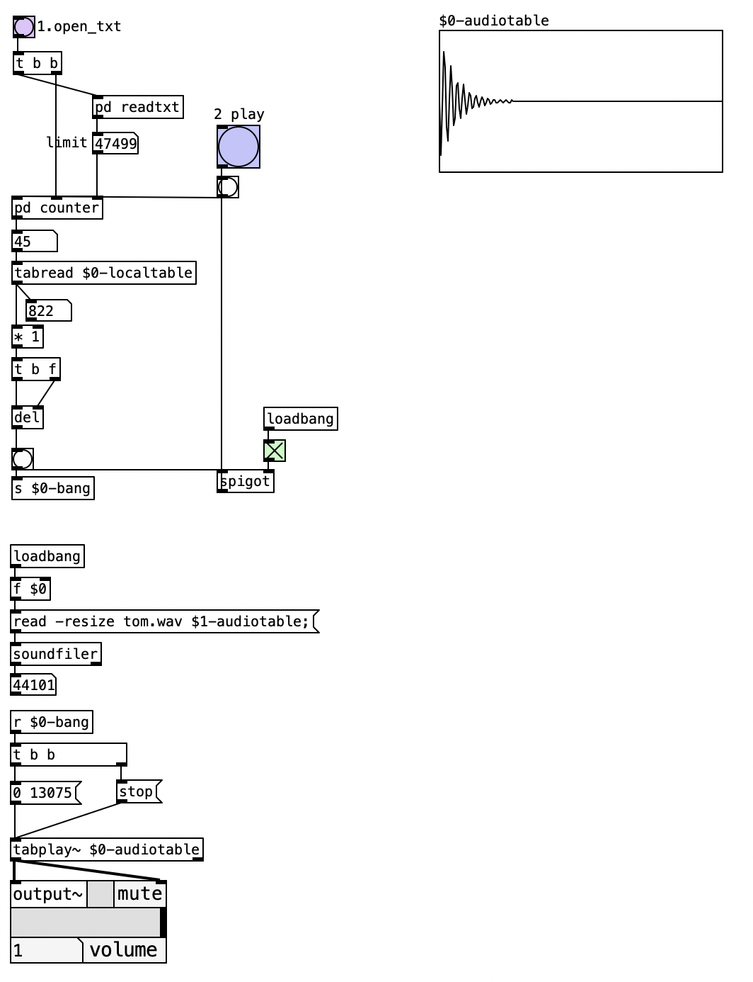
The readtxt subpatch functions as the primary data interface, managing both file loading and data quantification:
- Opens and reads the electrocardiogram.txt file
- Counts total data points for array sizing
- Loads data into local table for sequential access
- Provides file path management and error handling
Counter Subpatch
The counter mechanism implements sequential data traversal with automatic cycling:
- Maintains current position in ECG dataset
- Increments through data points on each trigger
- Resets to beginning when reaching data endpoint
- Provides configurable upper limits for partial data playback
5.7.2 Data Flow
graph TD
    A[electrocardiogram.txt] --> B[readtxt subpatch]
    B --> C[counter subpatch]
    C --> D[ECG Value Reader]
    D --> E[BPM Scaling]
    E --> F[Delay Object]
    F --> G[Bang Trigger]
    G --> H[Audio Playback]
    I[Audio File] --> J[audiotable Array]
    J --> K[tabplay~ Object]
    G --> K
    K --> L[Audio Output]
The ECG-controlled step sequencer shows a multi-stage data transformation process that converts static cardiac measurements into dynamic rhythmic triggers. This system demonstrates how biological timing patterns can be extracted and repurposed as musical control data, creating compositions that maintain organic temporal characteristics while serving structured musical functions.
The initial data preparation phase centers on the comprehensive loading and organization of the electrocardiogram dataset. The readtxt subpatch performs dual functions: it analyzes the text file structure to determine data quantity and simultaneously loads the numerical values into Pd’s table system for efficient random access. This preprocessing ensures that the cardiac data becomes immediately available for real-time sequential reading without file system delays that would disrupt musical timing. The subpatch communicates essential metadata to the main patch, including total data point count and successful loading confirmation, enabling the counter system to establish appropriate cycling boundaries for continuous operation.
The rhythmic control generation stage represents the core innovation where cardiac data becomes musical timing information. The counter subpatch maintains a position index that advances through the ECG dataset on each bang trigger, creating a sequential reading mechanism that treats the physiological data as a tempo map. Each ECG value retrieved through tabread undergoes scaling multiplication to convert the raw cardiac measurement into a meaningful delay time for the del object. This scaling factor determines the relationship between cardiac electrical activity levels and musical tempo, allowing for both literal interpretations where higher cardiac values produce faster rhythms, or inverted mappings where increased cardiac activity corresponds to longer inter-beat intervals, mimicking cardiac refractory periods.
The audio playback coordination stage transforms the ECG-derived timing signals into actual sound events through sophisticated sample triggering mechanisms. Each bang generated by the delay object initiates playback of audio material stored in the audiotable array via the tabplay~ object. The soundfiler object ensures that external audio files are properly loaded and resized within the array structure, while the spigot gate provides manual control over the sequencer’s operational state. This architecture enables the system to function as a complete musical instrument where the natural variability of cardiac rhythms generates complex polyrhythmic patterns that would be difficult to achieve through conventional programmed sequencing methods.
graph LR
    A[ECG Data Loading] --> B[Sequential Access]
    B --> C[BPM Conversion]
    C --> D[Delay Generation]
    D --> E[Audio Triggering]
5.7.3 Processing Chain Details
The patch maintains sonic coherence through several design considerations: the scaling factor allows adjustment of the overall tempo range to match rhythmn contexts, the counter’s cycling behavior ensures continuous operation without interruption, and the audio loading system supports various sample types from percussive hits to sustained tones. This flexibility enables the ECG step sequencer to function across diverse sound applications, from experimental compositions exploring biological rhythms to dance music productions requiring organic timing variations.
| Stage | Input | Process | Output |
|---|---|---|---|
| 1 | Text File | Data parsing and counting | Array population |
| 2 | Array Position | Sequential value retrieval | Raw ECG values |
| 3 | ECG Values | Multiplication scaling | Delay times (ms) |
| 4 | Delay Times | Temporal scheduling | Bang triggers |
| 5 | Bang Triggers | Audio sample initiation | Sound output |
5.7.4 Key Objects and Their Roles
| Object | Function | Parameters |
|---|---|---|
readtxt |
ECG data file reader | Loads and counts data points from text file |
counter |
Sequential data access | Steps through ECG values line by line |
tabread |
Array value retrieval | Reads individual ECG measurements |
del |
Rhythmic timing control | Creates delays based on ECG-derived BPM |
tabplay~ |
Audio sample playback | Triggers audio file samples |
soundfiler |
Audio file loader | Loads external audio into array |
5.7.5 Creative Applications
- Cardiac rhythm layering: Load different ECG datasets from multiple subjects to create polyrhythmic compositions where each person’s heartbeat triggers different audio samples
- Medical data sonification: Use ECG data from various cardiac conditions (arrhythmia, tachycardia, bradycardia) to generate distinct rhythmic patterns for educational or artistic purposes
- Biometric beat matching: Sync live performances to pre-recorded cardiac rhythms, creating music that literally follows the pulse of the performer or subject
- Physiological drum machines: Replace traditional step sequencer programming with real cardiac data to generate organic, non-repetitive percussion patterns
- Heart rate variability exploration: Use ECG datasets recorded during different emotional states or physical activities to trigger corresponding audio textures
- Interactive health installations: Design gallery pieces where visitors’ real-time heart rates control sample playback, creating personalized sonic experiences
- Temporal scaling experiments: Multiply ECG values by extreme factors to compress hours of cardiac data into minutes of rapid-fire triggering or extend brief arrhythmias into extended compositions
- Collaborative cardiac compositions: Network multiple ECG step sequencers where participants’ combined heart rhythms create collective musical pieces that reflect group physiological states
5.8 Image Sonification with RGBA Data
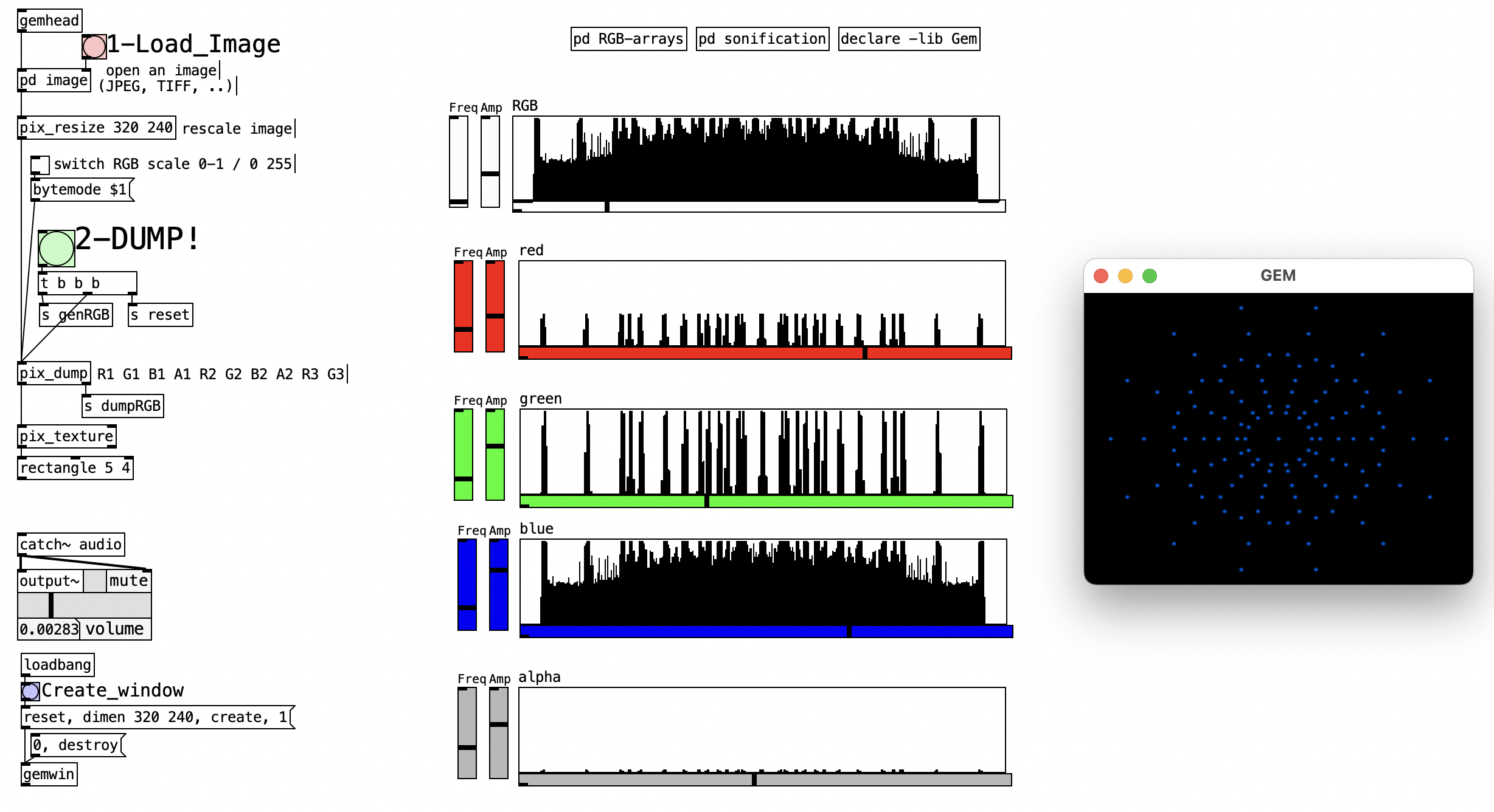
Digital images contain vast amounts of visual information encoded as pixel data, where each pixel represents color values across different channels. The RGBA image sonification patch transforms this visual data into auditory experiences by converting pixel color values into audio samples. This approach creates a direct mapping between visual and auditory domains, where the Red, Green, Blue, and Alpha channels of an image become independent audio streams that can be manipulated and mixed in real-time.
The sonification process reveals hidden patterns and textures within images that may not be immediately apparent through visual inspection alone. By treating pixel data as audio samples, we can explore the rhythmic, harmonic, and textural qualities inherent in visual compositions, creating a synesthetic bridge between sight and sound.
5.8.1 Patch Overview
The RGBA image sonification system consists of three main components working in concert:
- Image Loading and Analysis: Handles file import and pixel data extraction
- RGB-arrays (Data Processing): Normalizes and stores channel data in arrays
- Sonification Engine: Converts pixel data to audio with real-time controls
The patch workflow follows a clear data pipeline: images are loaded and decomposed into RGBA channels, pixel values are normalized and stored in arrays, and finally converted to audio samples with frequency and amplitude modulation capabilities.
5.8.1.1 Critical Data Processing Objects
pix_dump: This object serves as the bridge between GEM’s visual processing and Pd’s audio domain. It outputs a continuous stream of RGBA values (typically 0-255 range) that represent the complete image dataset.
Array Management: Each RGBA channel requires its own array for independent manipulation. The arrays store normalized values (-1 to 1) making them suitable for direct audio interpretation.
tabread4~: Provides crucial interpolation between array values, creating smooth audio transitions rather than harsh digital stepping when reading pixel data as audio samples.
5.8.2 Data Flow
flowchart TD
    A[Image File] --> B[pix_dump]
    B --> C[RGBA Pixel Stream]
    C --> D[RGB-arrays Subpatch]
    D --> E[Normalized Arrays R,G,B,A]
    E --> F[Sonification Subpatch]
    F --> G[Audio Output]
    H[Frequency Control] --> F
    I[Amplitude Control] --> F

    style A fill:#e1f5fe
    style G fill:#f3e5f5
    style D fill:#fff3e0
    style F fill:#fff3e0
The RGBA image sonification patch implements a comprehensive data transformation pipeline that converts visual information into auditory experiences through multiple interconnected processing stages. This workflow demonstrates how digital image data can be systematically decomposed, analyzed, and reconstituted as meaningful sonic representations while preserving the essential characteristics of the original visual content.
The initial image decomposition stage establishes the foundation for the entire sonification process through the critical function of the pix_dump object. When an image file is loaded into the system, whether in JPEG, PNG, TIFF, or other supported formats, the pix_dump object performs a comprehensive analysis that extracts every pixel’s color information as a sequential stream of numerical values. This extraction process follows a systematic pattern where each pixel contributes four distinct values representing its Red, Green, Blue, and Alpha channel intensities. The resulting data stream takes the form of R1 G1 B1 A1 R2 G2 B2 A2 R3 G3 B3 A3, creating a linear representation of the two-dimensional visual information. This linearization process effectively flattens the spatial relationships of the image into a temporal sequence, transforming visual space into a time-based data structure suitable for audio processing. The pixel values extracted during this stage typically range from 0 to 255, representing the standard 8-bit color depth used in most digital image formats.
The channel separation and normalization stage represents a critical transformation where the raw pixel data becomes suitable for audio synthesis applications. The continuous RGBA stream generated by the image decomposition process undergoes systematic demultiplexing, where individual color channel values are separated and directed into dedicated processing pathways. This separation enables independent manipulation of each color channel, allowing for sophisticated sonic textures that can emphasize specific visual characteristics of the original image. The Red channel array captures the warm color information and often contains significant luminance data, while the Green channel typically holds the most visually sensitive information due to human perception characteristics. The Blue channel frequently contains fine detail and cooler color information, and the Alpha channel represents transparency data that may reveal composition and layering information within the original image. Each separated channel undergoes normalization processing that converts the original 0-255 range into the -1 to 1 range required for audio synthesis, ensuring that the pixel data can be directly interpreted as audio sample values without amplitude clipping or distortion.
The audio synthesis stage transforms the normalized pixel arrays into dynamic audio streams through sophisticated control mechanisms that enable real-time manipulation of the sonification parameters. Each of the four normalized arrays becomes an independent audio source controlled by tabread4~ objects that perform interpolated reading of the stored pixel data. The frequency parameter, typically ranging from 0.1 to 20 Hz, determines the rate at which the system traverses through the pixel data, effectively controlling the temporal scaling of the visual information. Lower frequency values in the 0.1 to 1 Hz range reveal macro-structures and overall compositional elements of the image, allowing listeners to perceive broad color transitions and major visual forms through gradual sonic evolution. Higher frequencies in the 5 to 20 Hz range expose fine details and textures, creating rapid sonic fluctuations that correspond to pixel-level variations in the original image. The amplitude control parameter provides independent volume adjustment for each RGBA channel, enabling dynamic balancing that can emphasize particular color information or create complex sonic textures through channel interaction. The array index parameter allows for positional control within the image data, enabling targeted exploration of specific regions or systematic scanning of the entire visual content.
The signal mixing stage represents the culmination of the sonification process, where the four independent audio channels combine to create a unified sonic representation of the original image. This mixing process employs configurable amplitude controls that enable sophisticated real-time adjustment of the channel balance, allowing users to isolate individual color channels for detailed analysis or create weighted combinations that emphasize particular visual characteristics. Individual channel isolation proves particularly valuable for understanding how specific color information contributes to the overall visual composition, while weighted mixing enables the creation of custom sonic interpretations that highlight particular aspects of the image content. Dynamic balance adjustment during playback allows for evolving sonic textures that can reveal temporal patterns within the visual data or create artistic interpretations that maintain connection to the source material while achieving aesthetic coherence. The mixing stage also incorporates safeguards against amplitude overflow and provides signal conditioning that ensures the final audio output remains within acceptable dynamic ranges for both analytical listening and artistic presentation contexts.
Throughout this entire data flow pathway, the system maintains precise correspondence between visual and auditory domains, ensuring that the sonification preserves meaningful relationships between image characteristics and sonic parameters. This fidelity enables the patch to serve both analytical purposes, where visual patterns can be detected through auditory analysis, and creative applications, where image data becomes source material for musical composition and sound design. The modular architecture of the data flow also supports extension and customization, allowing users to insert additional processing stages or modify the parameter mappings to achieve specific analytical or artistic objectives.
The data transformation process involves several critical stages:
5.8.2.1 Stage 1: Image Decomposition
flowchart LR
    A[Image File] --> B[pix_dump] --> C[R1 G1 B1 A1 R2 G2 B2 A2 R3 G3 B3 A3]
5.8.2.2 Stage 2: Channel Separation and Normalization
flowchart LR
    A[RGBA Stream] --> B[Channel Demux]
    B --> C[Red Array]
    B --> D[Green Array]
    B --> E[Blue Array]
    B --> F[Alpha Array]

    C --> G[Normalize -1 to 1]
    D --> H[Normalize -1 to 1]
    E --> I[Normalize -1 to 1]
    F --> J[Normalize -1 to 1]
5.8.2.3 Stage 3: Audio Synthesis
Each normalized array becomes an audio source with independent control parameters:
| Parameter | Control Range | Audio Effect |
|---|---|---|
| Frequency | 0.1 - 20 Hz | Playback speed through pixel data |
| Amplitude | 0 - 1 | Volume level for each RGBA channel |
| Array Index | 0 - Array Size | Position within image data |
5.8.2.4 Stage 4: Signal Mixing
The four audio channels (RGBA) are mixed using configurable amplitude controls, allowing for: - Individual channel isolation - Weighted mixing of color information - Dynamic balance adjustment during playback
5.8.3 Key Objects and Their Roles
| Object | Function | Role in Sonification |
|---|---|---|
pix_dump |
Pixel data extraction | Converts image to sequential RGBA values |
array |
Data storage | Holds normalized pixel values for each channel |
tabread4~ |
Array interpolation | Smooth audio sample reading with interpolation |
phasor~ |
Timing control | Generates read position for array traversal |
*~ |
Audio mixing | Amplitude control and channel mixing |
dac~ |
Audio output | Final audio rendering |
5.8.4 Creative Applications
- Visual Music Composition: Transform paintings, photographs, or digital art into musical compositions where visual elements directly correlate to audio characteristics
- Color-Sound Synesthesia: Explore the relationship between color perception and auditory experience through real-time sonification
- Interactive Installations: Create responsive environments where visual input generates immediate audio feedback
- Pattern Recognition: Audio playback can reveal repetitive structures, gradients, and textures in images that may be difficult to perceive visually
- Data Archaeology: Sonify hidden or corrupted image data to identify patterns or anomalies
- Comparative Analysis: Compare multiple images by listening to their sonified representations
5.8.5 Technical Considerations
Frequency Scaling: The frequency control determines how quickly the system traverses through the pixel data. Lower frequencies (0.1-1 Hz) reveal macro-structures and overall image composition, while higher frequencies (5-20 Hz) expose fine details and textures.
Channel Weighting: Different RGBA channels contribute varying amounts of perceptual information:
- Red channel often contains luminance information
- Green channel typically has the highest visual sensitivity
- Blue channel may contain fine detail information
- Alpha channel represents transparency data
Array Size Optimization: Large images produce extensive arrays that may require memory management considerations. The patch can be optimized for specific image dimensions based on available system resources.
5.8.6 Performance Tips
- Start with low frequencies (0.1-0.5 Hz) to understand overall image structure
- Isolate individual channels to understand their unique contribution to the image
- Use amplitude controls to balance channels based on their visual prominence
- Experiment with different image types - photographs, abstract art, and technical diagrams produce distinctly different sonic characteristics
This sonification approach opens new possibilities for cross-modal artistic expression and analytical exploration, demonstrating how Pd’s flexible architecture enables innovative connections between disparate data domains.
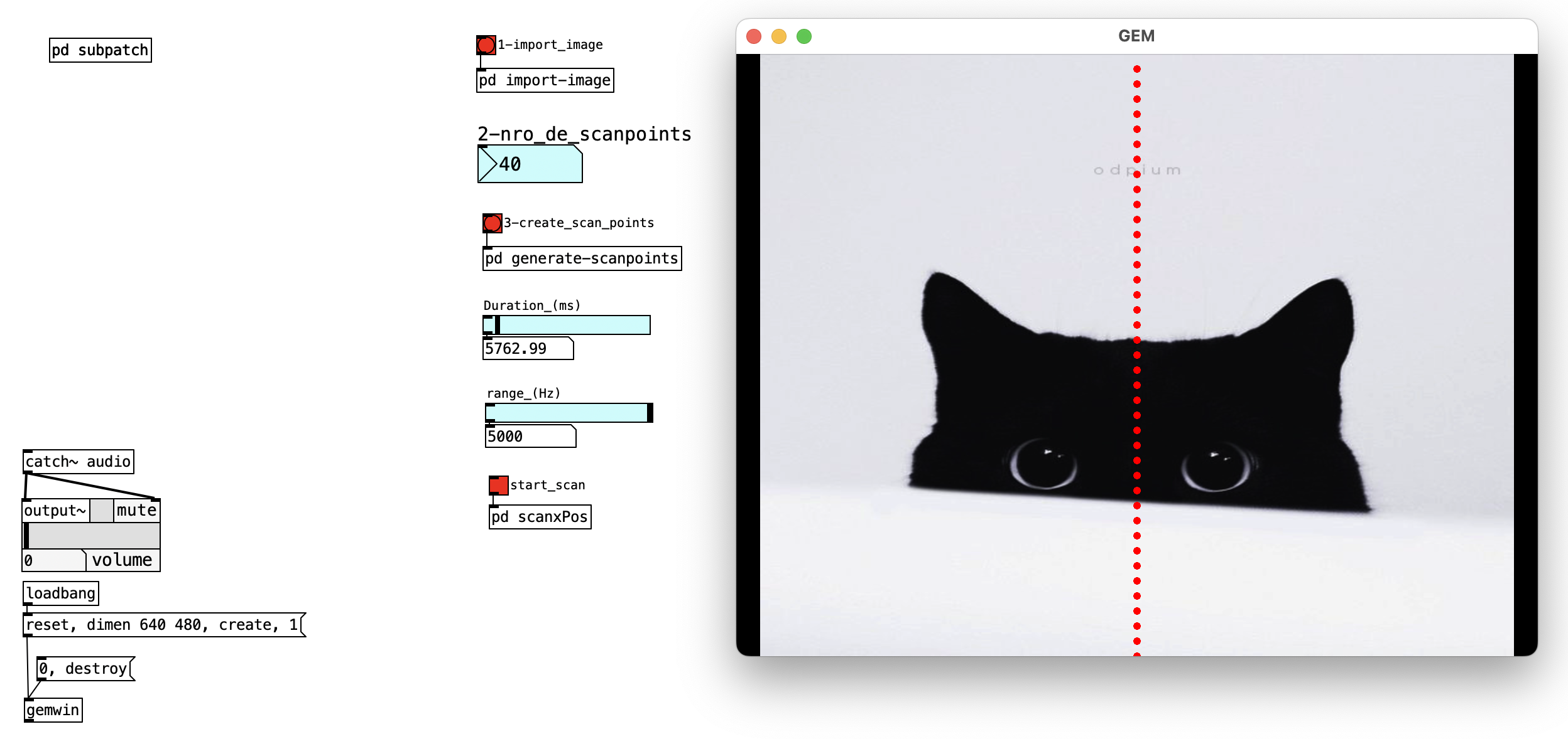
5.9 Image Scanner
This patch implements a linear scanning sonification that transforms visual image data into audio through systematic pixel sampling. By creating multiple scan points that traverse an image from left to right, the patch converts spatial color information into frequency-controlled oscillators, creating a real-time audio representation of visual content. This approach enables users to “hear” images through systematic exploration of pixel data across defined scan lines.
The scanning process reveals the vertical distribution of visual information within images, where different scan lines capture distinct horizontal slices of the visual content. Each scan point operates independently, creating polyphonic textures that reflect the complexity and variation present in the source image.
5.9.1 Patch Overview
The linear image scanner consists of four primary subsystems that work together to create a comprehensive image-to-audio conversion pipeline:
- Image Loading and Display: Manages file import and visual presentation through GEM
- Dynamic Scan Point Generation: Creates configurable numbers of scanning instances
- Pixel Data Extraction: Samples color values at specific image coordinates
- Audio Synthesis: Converts pixel data into frequency-controlled oscillators
The patch employs dynamic patching techniques to generate scalable numbers of scan points, each implemented as an instance of the linear-scan abstraction. This modular approach enables flexible configuration while maintaining efficient processing of multiple simultaneous scan lines.
5.9.1.1 Critical Processing Components
pix_data Object: This GEM object serves as the core interface between visual and audio domains. It samples pixel color values at specified x,y coordinates within the loaded image. The normalize message controls coordinate interpretation: when enabled (default), coordinates range from (0.0, 0.0) at bottom-left to (1.0, 1.0) at top-right; when disabled, coordinates use actual pixel dimensions.
Dynamic Patch Generation: The generate-scanpoints subpatch implements dynamic patching techniques to create configurable numbers of linear-scan instances. This system calculates y-position arguments for each scan line and generates the corresponding patch objects programmatically.
linear-scan Abstraction: Each scan line is implemented as an abstraction that receives a y-position argument determining its vertical position within the image. The abstraction contains the pixel sampling logic and frequency mapping calculations specific to that scan line.
5.9.2 Data Flow
flowchart TD
    A[Image File] --> B[pix_image/pix_texture]
    B --> C[Visual Display]
    D[Number of Scan Points] --> E[Dynamic Patch Generation]
    E --> F[linear-scan Abstractions]
    F --> G[pix_data Objects]
    G --> H[Pixel Color Extraction]
    H --> I[Frequency Mapping]
    I --> J[Oscillator Control]
    J --> K[Audio Output]
    L[Scan Duration Control] --> M[Temporal Coordination]
    M --> F

    style A fill:#e1f5fe
    style K fill:#f3e5f5
    style E fill:#fff3e0
    style F fill:#fff3e0
The linear image scanner a real-time processing pipeline that transforms static visual information into dynamic audio representations through systematic pixel sampling and frequency mapping. This process demonstrates how spatial image data can be converted into temporal audio experiences while preserving meaningful relationships between visual characteristics and sonic parameters.
The image loading and preparation stage establishes the foundation for the entire scanning process through comprehensive file management and visual processing setup. When an image file is loaded via the import-image subpatch, the system employs GEM’s pix_image object to read various image formats including JPEG, PNG, and TIFF into Pd’s visual processing environment. The loaded image undergoes texture processing through the pix_texture object, which prepares the pixel data for efficient random access while simultaneously enabling visual display within the GEM rendering window. This dual functionality ensures that users can see the image being processed while the scanning system extracts pixel information for audio synthesis. The image data becomes available to multiple pix_data objects that will sample specific pixel locations, with the texture object maintaining the image in memory for continuous access throughout the scanning process.
The dynamic scan point generation stage represents a sophisticated implementation of Pd’s dynamic patching capabilities, enabling user-configurable scanning resolution. The generate-scanpoints subpatch analyzes the user-specified number of scan points and calculates the appropriate y-coordinate distribution across the image height. For each scan point, the system generates a new instance of the linear-scan abstraction with a specific y-position argument that determines where that scan line will sample pixels vertically within the image. This y-position argument undergoes normalization calculation to ensure proper distribution from 0.0 (bottom of image) to 1.0 (top of image), creating evenly spaced scan lines that cover the entire vertical dimension of the source image. The dynamic generation process creates the necessary patch connections and initializes each scan line instance with its unique vertical position parameter, enabling parallel processing of multiple image regions simultaneously.
The pixel sampling and coordinate management stage implements the core data extraction functionality where visual information becomes available for audio processing. Each linear-scan abstraction contains a pix_data object configured to sample pixels at its assigned y-coordinate while the x-coordinate varies continuously during the scanning process. The temporal control system coordinates the scanning motion through line objects that interpolate x-position values from 0.0 to 1.0 over the user-specified scan duration. This creates synchronized left-to-right motion across all scan lines, with each line sampling pixels at its fixed y-position while traversing the full width of the image. The pix_data objects output both grayscale and RGB color values for each sampled pixel, providing multiple data streams that can be used for different aspects of the audio synthesis process. The temporal coordination ensures that all scan lines move in synchronization, creating coherent scanning motion that preserves the spatial relationships present in the original image.
The frequency mapping and audio synthesis stage transforms the extracted pixel data into meaningful audio parameters through sophisticated scaling and oscillator control. Each scan line’s pixel sampling output undergoes frequency mapping that converts color intensity values into specific frequency ranges for audio oscillators. The frequency distribution system maps the y-position of each scan line to a specific frequency band, creating a spectral arrangement where scan lines at the bottom of the image control lower frequencies while scan lines at the top control higher frequencies. This vertical frequency mapping creates intuitive correspondence between image position and audio pitch, enabling listeners to perceive spatial relationships within the image through pitch relationships in the audio output. The pixel intensity values modulate the oscillator frequencies within each scan line’s assigned frequency band, so brighter pixels produce higher frequencies while darker pixels produce lower frequencies within that band. Multiple oscillators operating simultaneously create polyphonic textures that reflect the complexity and variation present across different regions of the source image.
flowchart LR
    A[Image Loading] --> B[Scan Point Generation]
    B --> C[Pixel Sampling]
    C --> D[Frequency Mapping]
    D --> E[Audio Synthesis]
5.9.3 Processing Chain Details
The scanning system maintains precise temporal and spatial coordination through several sophisticated control mechanisms:
| Stage | Input | Process | Output |
|---|---|---|---|
| 1 | Image File | GEM loading and texture preparation | Accessible pixel data |
| 2 | Scan Point Count | Dynamic abstraction generation | Multiple linear-scan instances |
| 3 | Time Position | Synchronized x-coordinate interpolation | Pixel sampling coordinates |
| 4 | Pixel Color Values | Intensity to frequency conversion | Oscillator control signals |
| 5 | Multiple Frequencies | Polyphonic audio mixing | Combined audio output |
5.9.3.1 Temporal Control Parameters
| Parameter | Control Range | Audio Effect |
|---|---|---|
| Scan Duration | 100-90000 ms | Speed of left-to-right traversal |
| Frequency Range | 100-5000 Hz | Span of available frequencies |
| Scan Point Count | 1-256 points | Number of simultaneous scan lines |
| Y-Position Distribution | 0.0-1.0 | Vertical spacing of scan lines |
5.9.3.2 Coordinate Mapping System
The patch implements sophisticated coordinate management that ensures proper spatial relationships between image pixels and audio parameters:
Spatial Mapping: Each scan line occupies a fixed y-coordinate determined by its position in the overall distribution, while x-coordinates vary temporally from left to right during scanning.
Frequency Allocation: The vertical position of each scan line determines its base frequency range, creating spectral separation that preserves spatial information in the audio domain.
Temporal Synchronization: All scan lines move simultaneously from left to right, maintaining spatial coherence while revealing temporal evolution of visual content.
5.9.4 Key Objects and Their Roles
| Object | Function | Role in Scanning |
|---|---|---|
pix_image |
Image loading | Loads image files into GEM processing chain |
pix_texture |
Texture rendering | Enables visual display and pixel access |
pix_data |
Pixel sampling | Extracts color values at specified coordinates |
linear-scan |
Scan line abstraction | Implements individual scanning instances |
osc~ |
Audio oscillator | Generates frequency-controlled sine waves |
line |
Temporal interpolation | Controls scanning position over time |
metro |
Timing control | Coordinates scan timing across instances |
5.9.5 Creative Applications
- Musical Score Scanning: Transform written musical notation into audio by scanning staff lines, converting note positions into corresponding pitches and rhythms
- Texture Analysis: Explore the sonic characteristics of different visual textures by scanning patterns, fabrics, or surface details to reveal their rhythmic and harmonic qualities
- Architectural Sonification: Scan building facades, floor plans, or structural diagrams to create audio representations of architectural spaces and proportions
- Data Visualization Audio: Convert scientific charts, graphs, and data visualizations into audio to provide alternative access methods for visually impaired users
- Artistic Collaboration: Enable visual artists to hear their compositions while creating, providing real-time audio feedback during the visual creative process
- Interactive Installations: Create gallery pieces where visitors can upload images and immediately hear their sonic representation through the scanning system
- Educational Tools: Teach concepts of frequency, spatial relationship, and data representation by demonstrating direct correlations between visual and audio domains
- Live Performance Integration: Use the scanner with live video feeds or real-time image manipulation to create dynamic audio responses to visual performance elements
- Astronomical Data Exploration: Scan telescope images, star charts, or planetary surfaces to create audio representations of cosmic phenomena and celestial structures
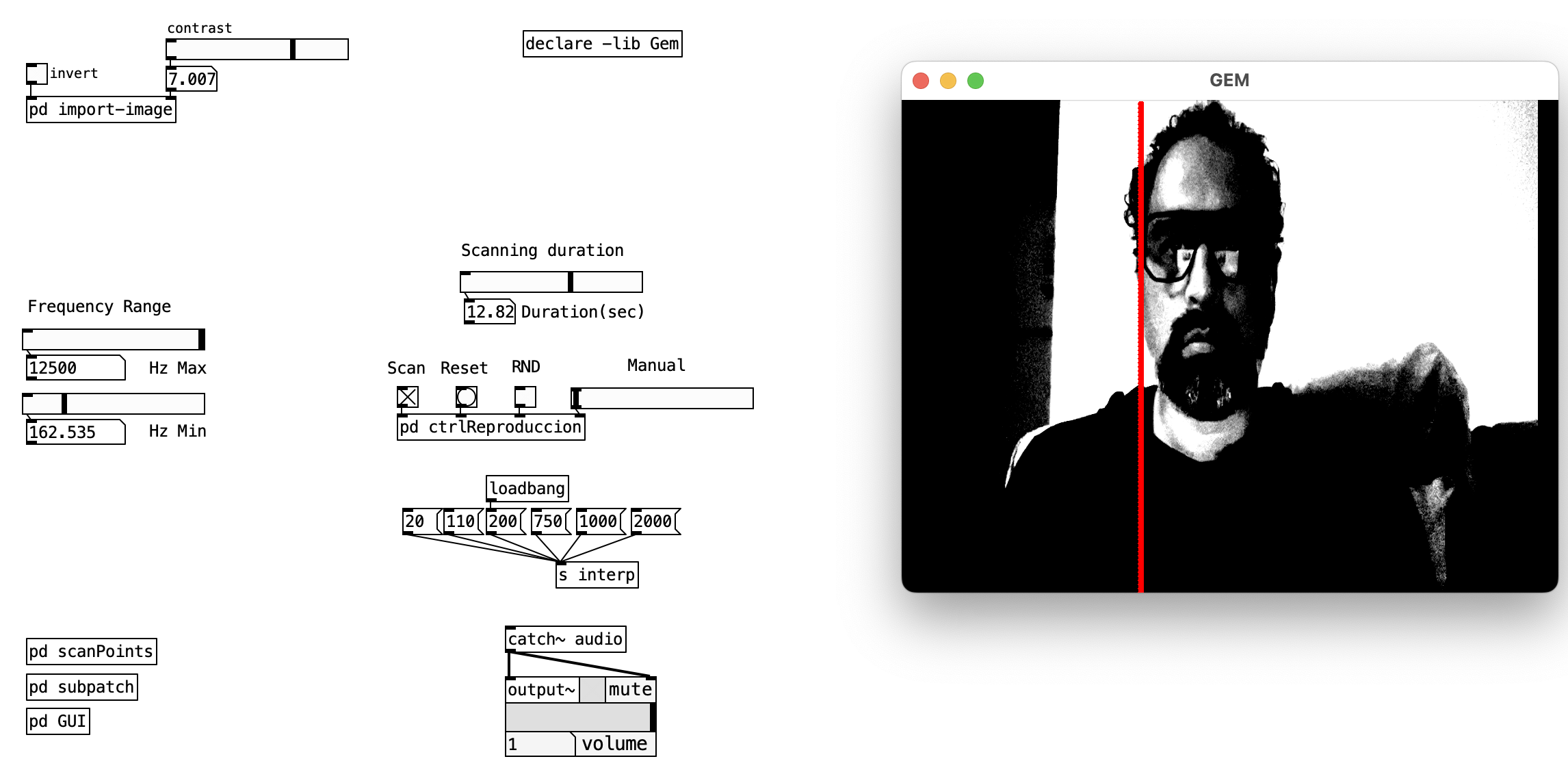
5.10 Camera Scanner
This patch extends the linear image scanning concept to real-time video input, creating dynamic sonification of live camera feeds. Unlike the static image scanner previously discussed, this patch processes continuous video streams from web cameras, enabling real-time exploration of moving visual content through audio. The patch maintains the core scanning methodology while introducing temporal dynamics that reflect the changing nature of live video input.
The live camera scanner transforms the temporal dimension of video into immediate sonic feedback, where movements, lighting changes, and scene transitions become audible through frequency modulation across multiple scan lines. This creates an interactive relationship between the physical environment captured by the camera and the generated audio landscape.
5.10.1 Patch Overview
The live camera scanner builds upon the established linear scanning framework while incorporating several enhancements specific to real-time video processing:
- Live Video Capture: Continuous camera input with adjustable contrast and color inversion
- Enhanced Scanning Controls: Random scanning modes and interpolated scan transitions
- Real-time Processing: Immediate response to visual changes in the camera feed
- Extended User Interface: Additional controls for camera manipulation and scanning behavior
The system maintains the same dynamic patching architecture and frequency mapping strategies established in the static image scanner, ensuring consistency in the sonification approach while adapting to the temporal nature of video input.
5.10.1.1 Live Video Processing Components
pix_video Object: Captures real-time video input from connected cameras, providing the continuous data stream that replaces static image loading. The object supports multiple camera devices and delivers frame-by-frame pixel data to the scanning system.
Image Enhancement Chain: The pix_2grey → pix_contrast → pix_invert processing chain offers real-time image manipulation capabilities that enhance the scanning process by adjusting visual characteristics to optimize sonic output.
Random Scanning System: Unlike static image scanning, the live camera scanner includes stochastic elements that introduce unpredictability to the scanning patterns, creating evolving audio textures that respond to both visual content and algorithmic variation.
5.10.2 Data Flow
The live camera scanner use a continuous real-time processing pipeline that transforms streaming video data into dynamic audio representations. While maintaining the core scanning methodology established in the static image scanner, this system introduces temporal continuity and enhanced control mechanisms that respond to the evolving nature of live video input.
The live video capture and preprocessing stage establishes a continuous data source through integrated camera management and image enhancement systems. The pix_video object maintains a persistent connection to the selected camera device, delivering frame-by-frame pixel data at standard video refresh rates. This continuous stream undergoes real-time preprocessing through a sophisticated image enhancement chain that optimizes the visual content for effective sonification. The pix_2grey object converts color video to grayscale, reducing computational complexity while preserving luminance information essential for frequency mapping. The pix_contrast object provides real-time contrast adjustment, enabling users to emphasize or diminish visual details based on scanning requirements. The optional pix_invert stage creates alternative visual representations that can reveal hidden patterns or provide aesthetic variations in the sonic output. This preprocessing chain ensures that the video data reaches the scanning system in an optimized format that maximizes the effectiveness of the pixel-to-frequency mapping process.
The enhanced scanning control stage introduces sophisticated temporal management systems that extend beyond the basic left-to-right scanning pattern. The system maintains the established dynamic scan point generation methodology while incorporating additional control mechanisms for temporal behavior. The random scanning subsystem employs random and spigot objects to introduce stochastic elements into the scanning pattern, creating unpredictable position variations that generate evolving audio textures independent of visual content changes. The scan interpolation system provides smooth transitions between scanning positions, reducing audio artifacts that might result from abrupt position changes in the video stream. The temporal coordination mechanisms ensure that all scan lines maintain synchronized motion while accommodating the additional complexity introduced by random positioning and interpolated movement patterns.
The real-time frequency mapping stage adapts the established pixel-to-frequency conversion methodology to accommodate the continuous nature of video input. Each scan line continuously samples pixels at its assigned y-coordinate while the x-coordinate evolves through the scanning pattern, creating ongoing frequency modulation that reflects both spatial relationships within the current video frame and temporal changes across successive frames. The frequency distribution system maintains the vertical mapping where scan lines at the bottom of the image control lower frequencies while scan lines at the top control higher frequencies, preserving the spatial-to-spectral correspondence established in the static scanner. However, the continuous nature of video input introduces temporal frequency modulation that creates evolving harmonic textures as visual content changes over time. The amplitude and frequency controls provide real-time adjustment capabilities that enable users to respond to changing lighting conditions, scene transitions, or desired aesthetic effects during live performance or analysis situations.
flowchart LR
    A[Live Video Input] --> B[Image Enhancement]
    B --> C[Dynamic Scanning]
    C --> D[Frequency Mapping]
    D --> E[Real-time Audio]
5.10.3 Processing Chain Details
The live camera scanner maintains the established processing architecture while incorporating real-time enhancements:
| Stage | Input | Process | Output |
|---|---|---|---|
| 1 | Camera Stream | Video capture and preprocessing | Enhanced video frames |
| 2 | Enhanced Frames | Dynamic scan point coordination | Synchronized scan positions |
| 3 | Scan Positions | Real-time pixel sampling | Continuous color values |
| 4 | Color Values | Live frequency mapping | Dynamic oscillator control |
| 5 | Audio Signals | Real-time mixing and output | Live audio stream |
5.10.3.1 Enhanced Control Parameters
| Parameter | Control Range | Live Scanning Effect |
|---|---|---|
| Contrast | 0-10 | Visual enhancement for improved frequency mapping |
| Random Scan | On/Off | Stochastic scanning pattern generation |
| Invert Colors | On/Off | Alternative visual representation |
| Scan Interpolation | Smooth/Linear | Transition quality between scan positions |
5.10.3.2 Real-time Performance Considerations
Frame Rate Coordination: The scanning system synchronizes with video frame rates to ensure smooth audio generation without dropouts or artifacts caused by timing mismatches between video capture and audio processing.
Adaptive Frequency Scaling: Real-time adjustment capabilities enable the system to respond to varying lighting conditions and scene content, maintaining optimal frequency mapping across different visual environments.
Computational Efficiency: The live processing requirements demand efficient algorithms that can maintain real-time performance while processing multiple scan lines simultaneously across continuous video streams.
5.10.4 Key Objects and Their Roles
Building upon the previously established scanning framework, the live camera scanner introduces several additional components:
| Object | Function | Role in Live Scanning |
|---|---|---|
pix_video |
Camera input capture | Provides continuous video stream from webcam |
pix_contrast |
Image enhancement | Adjusts pixel intensity for better scanning contrast |
pix_invert |
Color inversion | Creates alternative visual representations |
pix_2grey |
Grayscale conversion | Simplifies color data for processing |
random |
Stochastic positioning | Generates unpredictable scan patterns |
5.10.5 Creative Applications
- Live Performance Visualization: Create real-time audio responses to performer movements, gestures, or choreographed actions captured by the camera system
- Environmental Sonification: Transform ambient visual environments into evolving soundscapes that reflect changing lighting, weather conditions, or natural phenomena
- Interactive Installation Experiences: Enable gallery visitors to influence the sonic environment through their physical presence and movements within the camera’s field of view
- Surveillance Audio: Convert security camera feeds into audio monitoring systems that provide auditory alerts for visual changes or movement detection
- Accessibility Applications: Provide real-time audio descriptions of visual environments for visually impaired users, translating spatial and temporal visual information into sonic representations
- Dance and Movement Analysis: Create audio feedback systems for movement training where dancers can hear the sonic representation of their spatial positioning and temporal dynamics
- Telepresence Audio: Enable remote participants to experience distant visual environments through real-time sonification of camera feeds from other locations
- Machine Vision Integration: Combine computer vision algorithms with live scanning to create responsive systems that sonify specific detected objects, faces, or movement patterns
References
Canossa, Alessandro, Luis Laris Pardo, Michael Tran, and Alexis Lozano Angulo. 2022. “From Data Humanism to Metaphorical Visualization–an Educational Game Case Study.” In International Conference on Human-Computer Interaction, 109–17. Cham: Springer.
Gresham-Lancaster, Scot. 2012. “Relationships of Sonification to Music and Sound Art.” AI and Society 27 (2): 207–12.
Hallnäs, Lars, and Johan Redström. 2001. “Slow Technology–Designing for Reflection.” Personal and Ubiquitous Computing 5: 201–12.
Kim, Nam Wook, Hyejin Im, Nathalie Henry Riche, Alicia Wang, Krzysztof Gajos, and Hanspeter Pfister. 2019. “Dataselfie: Empowering People to Design Personalized Visuals to Represent Their Data.” In Proceedings of the 2019 CHI Conference on Human Factors in Computing Systems, 1–12. New York, NY, USA: Association for Computing Machinery.
Lupi, Giorgia. 2017. “Data Humanism: The Revolutionary Future of Data Visualization.” PrintMag. https://www.printmag.com/article/data-humanism-future-of-data-visualization/.