6  Spatial Audio

In the realm of sound, the concept of space is often overlooked. Yet, it plays a crucial role in shaping our auditory experience. The spatial dimension of sound is not merely an acoustic phenomenon; it is a fundamental aspect of how we perceive sound. This chapter explores the multifaceted nature of sound space, its historical evolution, and its implications for contemporary electroacoustic music.

6.1 The Music Sound Space

Sound always unfolds within a specific time and space. From the very moment sound is generated in music, space is implicitly present, enabling the possibility of organizing, reconstructing, and shaping that space to influence musical form. Thus, the use of space in music responds to concerns that go far beyond mere acoustic considerations.

Conceiving space as a structural element in the construction of sonic discourse requires us to address a complex notion—one that touches on multiple dimensions of composition, performance, and perception. This idea rests on the argument that space is a composite musical element, one that can be integrated into a compositional structure and assume a significant role within the formal hierarchy of sound discourse.

Spatiality in music represents a compositional variable with a long historical lineage. The treatment of sound space on stage can be traced back to classical Greek theatre, where actors and chorus members used masks to amplify vocal resonance and enhance vocal directionality (Knudsen 1932). However, while compositional techniques addressing spatial sound have been developing for centuries, it is not until the early 20th century that a systematic use of spatial dimensions becomes central to musical structure. Landmark works such as Universe Symphony (1911–51) by Charles Ives, Déserts (1954) and Poème électronique (1958) by Edgard Varèse, Gruppen (1955–57) by Karlheinz Stockhausen, and Persephassa (1969) by Iannis Xenakis approach spatiality as an independent and structural dimension. In these works, space is interrelated with other sonic parameters such as timbre, dynamics, duration, and pitch.

Particularly noteworthy is that these pieces do not merely establish sonic space as a new musical dimension—they also develop theoretical frameworks for the spatialization of sound. These theories consider physical, poetic, pictorial, and perceptual aspects of spatial sound. As a result, in recent decades the areas of research and application related to artistic-musical knowledge have expanded significantly, fostering interdisciplinary inquiry into sound space and its parameters.

Beyond its central role in music, in recent years spatial sound has also become a subject of study across a variety of disciplines. One example of this is found in research into sound spatialization techniques in both real and virtual acoustic environments. These techniques have largely evolved based on principles of psychoacoustics, cognitive modeling, and technological advancements, leading to the development of specialized hardware and software for spatial sound processing. In the scientific realm, theses and research articles have explored, in great detail, the cues necessary to create an acoustic image of a virtual source and how these cues must be simulated—whether by electronic circuitry or computational algorithms.

However, it must be noted that musical techniques for managing sound space have not yet fully integrated findings from perceptual science. As we will explore later, many artistic approaches rely on only a subset of the cues involved in auditory spatial perception, overlooking others that are essential for producing a convincing acoustic image.

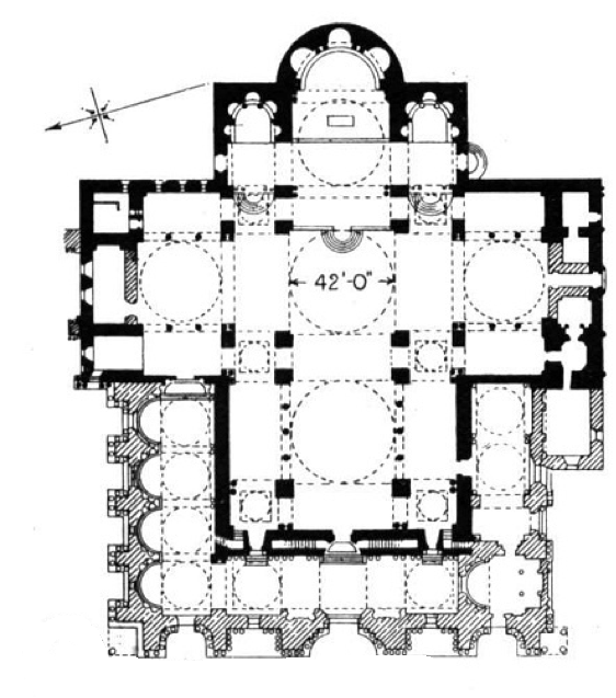
In general terms, the spatial dimension of a musical composition can function as the primary expressive and communicative attribute for the listener. For instance, from the very first moment, the acoustic characteristics of a venue—real or virtual—directly affect how we perceive the sonic discourse. This dimension of musical space is further shaped by the placement of sound sources, whether instrumentalists or loudspeakers. A historical precedent for this can be found in the Renaissance period through the use of divided choirs in the Basilica of San Marco in Venice. This stylistic practice, known as antiphonal music, represents a clear antecedent of the deep connection between musical construction and architectural space (Stockhausen 1959). The style of Venetian composers was strongly influenced by the acoustics and architectural features of San Marco, involving spatially separated choirs or instrumental groups performing in alternation.

Floor plan of the Basilica of San Marco in Venice (Italy).

6.1.1 Spatial Distribution and the Evolution of Listening Spaces

During the European Classical and Romantic periods, the spatial distribution of musicians generally adhered to the French ideal inspired by 19th-century military band traditions. In this widely adopted setup, space was typically divided into two main zones: musicians arranged on a frontal stage and the audience seated facing them. This concert model—linear, frontal, and fixed—reflected a formalized, hierarchical approach to the musical experience.

By the 20th century, this front-facing paradigm began to be reexamined and reimagined. Composers and sound artists started to question the limitations of conventional concert hall layouts. A notable example is found in 1962, when German composer Karlheinz Stockhausen proposed a radical redesign of the concert space to accommodate the evolving needs of contemporary composition. His vision included a circular venue without a fixed podium, flexible seating arrangements, adaptable ceiling and wall surfaces for mounting loudspeakers and microphones, suspended balconies for musicians, and configurable acoustic properties. These directives were not merely architectural; they were compositional in nature, meant to transform the listening experience by embedding spatiality into the core of musical structure.

This reconceptualization of space enabled a new way of thinking about the sensations and experiences that could be elicited in the listener through the manipulation of spatial audio. The concert hall was no longer a passive container of sound, but an active participant in its articulation.

In parallel developments, particularly in the field of electroacoustic music during the mid-20th century, spatial concerns were often shaped by the available technology of the time. Spatiality lacked a clearly defined theoretical vocabulary and was not yet integrated systematically with other familiar musical parameters. Nonetheless, from its inception, electroacoustic music leveraged technology to expand musical boundaries—either through electronic signal processing or by interacting with traditional instruments.

However, the notion of space in electroacoustic music differs significantly from that of instrumental music. In this context, spatiality is broad, multidimensional, and inherently difficult to define. It encompasses not only the individual sonic identity of each source—typically reproduced through loudspeakers—but also the relationships between those sources and the acoustic space in which they are heard. Critically, the audible experience of space unfolds through the temporal evolution of the sonic discourse itself.

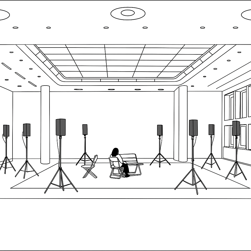
Loudspeakers in electroacoustic music afford a uniquely flexible means of organizing space as a structural element. The spatial potential enabled by electroacoustic technologies has been, and continues to be, highly significant. With a single device (see Fig. 2), it is possible to transport the listener into a wide range of virtual environments, expanding the scope of musical space beyond the physical limitations of the performance venue. This opens the door to sonic representations of distance, movement, and directionality—factors that can be fully integrated into the musical structure and treated as compositional dimensions in their own right.

Multichannel electroacoustic concert hall.

6.1.2 Spatial Recontextualization and Auditory Expectation

One of the defining characteristics of electroacoustic music is its capacity to recontextualize sound. Through virtual spatialization, a sound can acquire new meaning depending on how it functions within diverse contexts. For example, two sounds that would never naturally coexist—such as a thunderstorm and a mechanical engine in the same acoustic scene—can be juxtaposed to create a landscape that defies ecological realism. This deliberate disjunction can trigger a complex interaction between what is heard and the listener’s prior knowledge of those sound sources, drawn from personal experience.

Our ability to interpret spatial cues in sound is deeply shaped by the patterns of interpersonal communication we engage in, the lived experience of urban or rural environments, and the architectural features of our surroundings. These formative influences are so embedded in our perceptual systems that we are often unaware of their role in shaping how we understand sensory information. Spatial cues are constantly processed in our everyday auditory experience and play a vital role in shaping our listening behaviors.

In the context of electroacoustic music, environmental cues may not only suggest associations with a physical location but also inform more abstract properties of the spatial discourse articulated by the piece. Jean-Claude Risset (Risett 1969) noted a tension in using environmental recordings in electroacoustic composition: the recognizable identity of “natural” sounds resists transformation without diminishing their spatial content. Nevertheless, identifiable sounds remain central to electroacoustic works, particularly those aligned with the tradition of musique concrète.

Under normal listening conditions, perception of a singular sound source is shaped by what Pierre Schaeffer (Schaeffer 2003) defined as the “sound object”—a sonic phenomenon perceived as a coherent whole, grasped through a form of reduced listening that focuses on the sound itself, independent of its origin or meaning. Our auditory system has evolved to identify and locate such sound objects in space by mapping them according to the physical attributes of their sources. A barking sound is understood as coming from a dog; a voice is mapped to a human speaker. As a result, the spatial interpretation of sound is closely linked to the listener’s expectations, shaped not only by the inherent acoustic characteristics of the signal but also by the listener’s accumulated learning and experience.

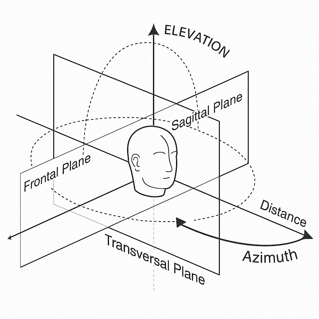
Unlike incidental listening in everyday life, attentive listening in electroacoustic music generally occurs from a fixed position. Apart from minor head movements, the spatial information available to the listener depends entirely on the acoustic cues encoded in the sound. While spatial hearing has been extensively researched in the field of psychoacoustics, its compositional potential as a carrier of musical form remains underexplored. In particular, the dimension of distance has received little attention compared to azimuth (horizontal angle) and elevation (vertical angle). These two spatial dimensions have been rigorously studied and well-documented, forming the basis of many standard models of spatial perception.

By contrast, the auditory perception of distance remains one of the most enigmatic topics in both music and psychophysics. It involves a complex array of cues—many of which are still not fully understood or integrated into compositional practice. As such, distance remains an open and promising field of inquiry for creative and scientific exploration alike (Abregú, Calcagno, and Vergara 2012).

Schematic representation of the azimuth, elevation, and distance axes.

6.1.3 The Expanded Spatial Palette of Electroacoustic Music

Unlike instrumental music, which relies on the physicality of pre-existing sound sources, electroacoustic music is not constrained by such limitations. This fundamental distinction allows composers not only to design entirely new sounds tailored to their spatial intentions but also to explore acoustic environments that defy conventional physical logic. While a performance of acoustic music offers visual and sonic cues grounded in the material world—a stage, a hall, visible instruments—electroacoustic music invites a more abstract engagement, where the listener navigates a virtual sound world.

In acoustic settings, physical space provides the listener with consistent spatial information. In contrast, electroacoustic environments—particularly those utilizing multichannel reproduction—radically extend the spatial canvas. These environments challenge and expand our auditory expectations, offering a broader spectrum of spatial strategies shaped by the interaction between sound diffusion technologies and the perceptual mechanisms of the listener.

Yet, this very potential also brings complications. The ephemeral and immaterial nature of loudspeaker-based sound makes it difficult to generate a spatial image as vivid or intuitive as that encountered in the physical world. Despite technological precision, virtual spatial environments often lack the tactile immediacy of real acoustic spaces.

Research in the field of computer music typically falls into two major domains: the study of spatial hearing and cognition, and the development of sound reproduction technologies. One of the advantages in electroacoustic contexts is the ability to isolate and manipulate spatial cues independently—a task nearly impossible with traditional acoustic instruments. This level of control opens up possibilities for treating space as a fully sculptable compositional parameter. However, practical results vary greatly, and many perceptual questions remain unresolved. It is within this intersection—where psychophysics, spatialization technologies, and compositional imagination meet—that the most fertile ground for innovation lies.

A classic example is John Chowning’s Turenas (1972), which employed quadraphonic speaker arrangements and a mathematical model to simulate virtual spatial motion. Chowning implemented a distance-dependent intensity multiplier according to the inverse square law, applied independently to each channel. The outcome was a virtual “phantom source” whose movement through space was dynamically shaped and perceptually engaging. Interestingly, Chowning discovered that simple, well-structured paths—such as basic geometric curves—produced the most convincing spatial gestures. In On Sonic Art (Wishart 1996), one finds multiple visual representations of two-dimensional spatial trajectories; however, these diagrams often fail to translate into equally perceptible auditory experiences. For instance, while Lissajous curves are visually complex and elegant, their perceptual distinctiveness can be minimal. Clarity, it turns out, is key to audible spatial expression.

Since the mid-20th century, various spatialization systems have emerged to simulate acoustic spaces through loudspeaker arrays. Among the most notable are Intensity Panning, Ambisonics, and Dolby 5.1. Although a detailed technical comparison of these systems lies beyond the scope of this section (see (Basso, Di Liscia, and Pampin 2009) for an extensive overview), it is worth noting that electroacoustic space only becomes meaningful if its structural characteristics—such as reverberation—can be clearly perceived. In orchestral music, spatial features are often inherent to the instrument layout and performance context. With fixed instrument positions, the spatial configuration is relatively stable. In virtual space, however, reverberation must be explicitly created and shaped to define the acoustic character of the environment in which sonic events unfold.

Unlike the relatively fixed reverberation properties of physical rooms, virtual spaces offer remarkable plasticity. Composers can craft distinct acoustic identities for different sections of a piece, allowing each space to function as a compositional agent in its own right. This flexibility implies that in electroacoustic music, space must often be invented—not merely inherited from the sounding objects, as is typically the case with acoustic instruments.

It becomes clear, then, that spatial design can be a powerful structural element in music. Sound space carries poetic, aesthetic, and expressive dimensions. At the same time, convincing spatial construction often depends on our embodied experience of real-world acoustics. This dual grounding—in perceptual realism and creative abstraction—opens new theoretical and practical avenues for artists. The potential to reconceptualize spatiality through an expanded compositional lens can empower creators to engage more fully with the multidimensionality of sonic art. In doing so, it enables the development of richer analytical and taxonomical criteria that extend beyond sound itself, embracing broader cultural, perceptual, and technological contexts.

6.2 Spatial Localization of Sound

When we perceive a sound event, we rely on a variety of auditory cues to infer the position of its source. These cues are associated with both direction and distance, and are typically classified into two main categories: binaural cues, which arise from comparisons between the two ears, and monaural cues, which are perceived by a single ear and are still critical for spatial localization.

To illustrate the binaural mechanism, consider a point sound source moving in a horizontal circular path around a listener’s head. At any given moment, the distance from the source to each ear will differ depending on the angular position of the source. This spatial configuration results in time and intensity differences between the two ears. These discrepancies are key to our spatial perception of sound.

When a sound wave reaches the right ear before the left, the slight delay in arrival time is known as the Interaural Time Difference (ITD), while the difference in loudness is called the Interaural Level Difference (ILD). These cues are extremely subtle—at 90°, the maximum ITD is around 630 microseconds—yet the brain is remarkably adept at interpreting them to infer the lateral position of the source.

The ILD is largely caused by the acoustic shadowing effect of the head. For higher frequencies (with wavelengths shorter than the head’s diameter), the sound cannot diffract around the head, leading to more pronounced differences in intensity between the ears, depending on the angle of incidence.

These binaural cues work together most effectively between 800 Hz and 1600 Hz. Below 800 Hz, ITD is the dominant cue; above 1600 Hz, ILD becomes more effective. The distance between the listener and the sound source also affects these cues, with ILD being particularly sensitive to distance changes, while ITD remains relatively stable.

Binaural localization does not require prior knowledge of the sound source. In contrast, monaural localization—when only one ear is used—often depends on recognizing the sound in advance. One key monaural cue is the Spectral Cue (also called the Monaural Spectral Cue), which arises from changes in the sound spectrum caused by interactions with the outer ear (the pinna).

Even slight modifications in the signals reaching the auditory system can lead to significant shifts in the perceived spatial image. From an acoustic perspective, the pinna acts as a directional filter, primarily affecting high frequencies. It introduces spectral and temporal modifications to the signal depending on its angle of incidence and distance. These effects help the listener distinguish between sounds originating in front versus behind, and also assist in determining the elevation of the source.

Historically, the role of the pinnae in spatial hearing was underestimated, often seen merely as protective structures. Contemporary research, however, confirms their essential role in spatial perception and in reducing environmental noise, such as wind.

When it comes to estimating source distance, familiarity with the sound plays a significant role. For example, spoken voice at a normal volume provides a relatively accurate cue for distance perception. Like light intensity or visual size, sound intensity decreases with distance, following the inverse square law. But intensity is not the only factor: air acts as a low-pass filter, attenuating high frequencies over distance. This effect is clearly noticeable in scenarios like an approaching airplane, where the sound not only grows louder but also becomes brighter and richer in frequency content.

In sum, sound localization is a complex perceptual process informed by a combination of binaural and monaural cues, spectral filtering by the outer ear, and familiarity with the sound source. These mechanisms interact continuously to allow listeners to orient themselves in a dynamic acoustic environment, whether real or simulated.

6.3 Hearing in Enclosed Spaces

When we experience sound in an enclosed environment, the first auditory cue that reaches our ears is known as the direct sound—the signal that travels straight from the source without interacting with any obstacles. This is followed by the first-order reflections, which occur when the sound bounces off a single surface—such as a wall—before reaching the listener. These are then succeeded by second-order reflections, involving two bounces, and progressively higher orders of reflection. Eventually, this cascade of reflections gives rise to a diffuse auditory sensation known as reverberation.

In a typical empty room—consider one with four walls, a ceiling, and a floor—the six primary surfaces contribute to the first-order reflections. These early reflections are particularly significant when the sound has a sharp or impulsive attack, as they assist the auditory system in identifying the spatial position of the sound source. Reverberation, by contrast, carries information about the acoustic properties and dimensions of the room. It plays a key role in shaping the overall perception of the space’s material and geometry.

A critical metric used in room acoustics is the reverberation time, commonly denoted as T₆₀. This refers to the time it takes for the reverberant sound energy to decay by 60 decibels after the original sound source has ceased. A widely used formula for estimating this value is the Sabine equation: \[T_{60} = 0.16 \times \frac{V}{A}\]

Here, V represents the volume of the room in cubic meters, and A is the total equivalent absorption area, calculated as the sum of the products of each surface’s area and its corresponding absorption coefficient. Importantly, absorption coefficients are frequency-dependent, meaning that the acoustic behavior of a room varies with different sound frequencies.

To account for this, acousticians often use a metric known as the Noise Reduction Coefficient (NRC), which averages absorption values across key frequencies—specifically 250 Hz, 500 Hz, 1000 Hz, and 2000 Hz. This provides a more practical estimate of how a room absorbs sound across the human auditory spectrum.

A graphical representation of room acoustics typically illustrates the temporal distribution of reflections produced by an impulse response within the space. In such plots, the height of each line corresponds to the relative amplitude of each reflection. These visualizations help researchers and designers understand how sound energy evolves over time in an architectural space, offering insight into both clarity and spatial impression.

Understanding how direct sound, early reflections, and reverberation interact is essential for both technical and artistic applications in sound design. Whether composing for multichannel electroacoustic environments or designing spatial sound installations, these acoustic principles are fundamental to crafting immersive and intelligible auditory experiences.

6.4 Virtual Source Simulation via Stereophonic Techniques

Stereophonic systems enable the simulation of virtual sound source localization using just two loudspeakers positioned to the left and right of the listener. By manipulating the amplitude of each signal sent to the speakers, we can generate the perceptual illusion of a sound source moving laterally across the auditory field. Additional transformations also allow us to simulate depth and even create the sensation of a source emanating from behind the speakers, constructing an illusory auditory space.

The perception of a virtual source positioned between two speakers arises from the system’s ability to artificially generate an Interaural Level Difference (ILD). If the signal emitted from the right speaker is louder than that from the left, the right ear perceives a higher intensity, prompting the auditory system to localize the source toward the right. The degree of perceived lateral displacement is directly proportional to the intensity difference.

In typical stereo setups, the speakers are arranged with a 60° separation. However, for purposes of spatial expansion and compatibility with quadraphonic systems (involving four speakers surrounding the listener), we assume a 90° separation. We define 0° as the location of the left speaker and 90° as the right. The objective is to calculate the appropriate amplitude for each speaker to position the virtual source at a desired angle θ within this range.

To ensure the virtual source appears equidistant from the listener during its movement, the total sound intensity emitted by both speakers must remain constant. That is:

\[ I_L + I_R = k \]

Assuming intensity is normalized between 0 and 1, we can simplify this to:

\[ I_L + I_R = 1 \]

Here, \(I_L\) and \(I_R\) represent the intensities emitted by the left and right speakers, respectively. When the source is fully localized at the left, \(I_L = 1\) and \(I_R = 0\); when at the right, \(I_L = 0\) and \(I_R = 1\); and when centered, both are \(0.5\). However, in most digital audio systems we operate on amplitude, not intensity. Since intensity is proportional to the square of amplitude, we use the relation:

\[ I \propto A^2 \]

Thus, the condition of constant intensity becomes:

\[ A_L^2 + A_R^2 = 1 \]

A common misconception is to linearly scale amplitudes (e.g., \(A_L = A_R = 0.5\) when centered), but this would yield:

\[ 0.5^2 + 0.5^2 = 0.25 + 0.25 = 0.5 \]

—only half the intended total intensity, which could be mistakenly perceived as an increase in distance. To preserve consistent intensity across the stereo field, we rely on a trigonometric identity:

\[ \sin^2(\theta) + \cos^2(\theta) = 1 \]

Using this, we can define the amplitude assignments as:

\[ A_R = \sin(\theta) \\ A_L = \cos(\theta) \]

Where θ ranges from 0° (left) to 90° (right). For example, at 45°, both \(sin(45^\circ)\) and \(cos(45^\circ)\) equal approximately 0.707. Squaring and summing these values confirms that the total intensity remains 1:

\[ A_R^2 + A_L^2 = \sin^2(45^\circ) + \cos^2(45^\circ) = 0.5 + 0.5 = 1 \]

Thus, this method preserves the perceptual coherence of the virtual sound source’s position while maintaining a constant energy output, a critical aspect of spatial audio realism.

In summary, for any virtual angle \(\theta \in [0^\circ, 90^\circ]\), we can accurately simulate spatial position with consistent intensity using:

\[ A_R = \sin(\theta) \\ A_L = \cos(\theta) \]

This technique forms the basis for further expansion into quadraphonic and multichannel spatialization systems.

6.5 Implementing a Stereo Spatialization in Pd

Before diving into the implementation of a stereophonic spatialization system in Pd, it is essential to note that the objects used to compute trigonometric functions such as sine and cosine require the input angle to be expressed in radians, not degrees. Recall that one radian is the angle formed when the length of the arc of a circle equals the radius. From this definition, we derive the following equivalences:

• 360° = \(2\pi\) radians
  
• 180° = \(\pi\) radians
  
• 90° = \(\frac{\pi}{2}\) radians

To convert degrees to radians, we multiply the angle in degrees by the ratio (\(\frac{2\pi}{360}\)). To optimize performance and avoid redundant calculations, we can precompute this factor:

\[ \text{Angle}_{\text{rad}} = \text{Angle}_{\text{deg}} \times \frac{2\pi}{360} = \text{Angle}_{\text{deg}} \times 0.0174533 \]

Intensity panning implementation with angular control and trigonometric amplitude distribution for stereophonic sound source positioning.

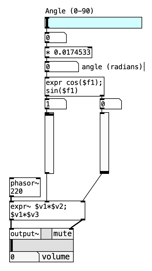
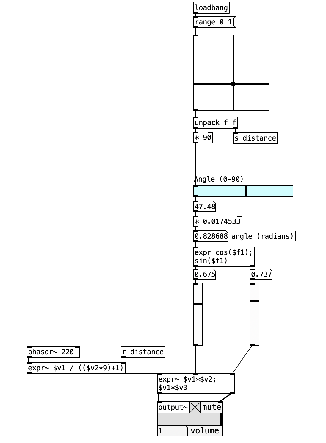
The patch illustrated below simulates a virtual sound source using stereophonic panning. This technique, commonly referred to as intensity panning, adjusts the balance between two loudspeakers. The source signa is split into two channels, each multiplied by the cosine and sine of the specified angle (in radians) to distribute the amplitude between the left and right speakers. As we vary the angle between 0° and 90°, the source appears to move along an arc, emulating the listener’s perception of spatial position.

This Pd patch shows the fundamental principles of stereophonic spatialization through intensity panning, implementing the mathematical framework for creating virtual sound source positioning between two speakers. By applying trigonometric amplitude control to left and right audio channels, the patch enables precise localization of monophonic sources within a 90-degree stereo field while maintaining constant total energy output. This approach forms the foundation for understanding spatial audio processing and serves as a building block for more complex multichannel spatialization systems.

The patch provides real-time control over angular positioning through intuitive slider interfaces, allowing users to experience the direct relationship between mathematical spatial calculations and perceptual sound localization. This implementation serves both educational and practical purposes, demonstrating how theoretical acoustic principles translate into functional audio processing tools.

6.5.1 Patch Overview

The intensity panning system implements a complete stereophonic spatialization pipeline consisting of four primary processing stages:

1. Angle Input and Conversion: Manages user input and degree-to-radian conversion
2. Trigonometric Calculation: Computes sine and cosine values for amplitude control
3. Audio Generation and Processing: Creates test signals and applies spatial positioning
4. Stereo Output: Delivers positioned audio to left and right channels

The patch demonstrates the essential mathematical relationship where spatial positioning is achieved through complementary amplitude control, ensuring that the virtual source maintains consistent perceived loudness while moving between speakers.

6.5.1.1 Critical Processing Components

Degree-to-Radian Conversion: The multiplication factor 0.0174533 represents the mathematical constant π/180, enabling conversion from user-friendly degree input to the radian values required by Pd’s trigonometric functions. This conversion ensures precise mathematical calculation while maintaining intuitive user control.

Trigonometric Expression: The expr cos($f1) \; sin($f1) object simultaneously calculates both amplitude coefficients needed for stereophonic positioning. The cosine output controls left channel amplitude, while sine controls right channel amplitude, creating the complementary relationship essential for constant-energy panning.

Audio Expression Multiplier: The expr~ $v1*$v2 \; $v1*$v3 object performs real-time multiplication of the audio signal with the calculated trigonometric values, applying the spatial positioning in the audio domain while maintaining sample-accurate timing.

6.5.2 Data Flow

flowchart TD
    A[Angle Input 0-90°] --> B[Degree to Radian Conversion]
    B --> C[Trigonometric Calculation]
    C --> D[Sine/Cosine Values]
    D --> E[Audio Signal Generation]
    E --> F[Amplitude Modulation]
    F --> G[Left Channel Output]
    F --> H[Right Channel Output]
    I[Test Oscillator] --> E
    
    style A fill:#e1f5fe
    style G fill:#f3e5f5
    style H fill:#f3e5f5
    style C fill:#fff3e0

The stereophonic intensity panning patch orchestrates a mathematical transformation pipeline that converts angular positioning information into spatially positioned audio output through systematic trigonometric processing. This implementation demonstrates how theoretical spatial audio principles translate into practical real-time audio processing systems that maintain both mathematical accuracy and perceptual coherence.

The angle input and preprocessing stage establishes the foundation for spatial positioning through user interface management and mathematical preparation. The horizontal slider (hsl) provides intuitive control over the desired angular position, accepting input values in the familiar degree scale from 0° to 90°, where 0° represents full left positioning and 90° represents full right positioning. This degree-based input undergoes immediate conversion to radians through multiplication by the constant 0.0174533 (π/180), transforming the user-friendly angular measurement into the mathematical format required by Pd’s trigonometric functions. The conversion process ensures that subsequent calculations maintain precision while preserving the intuitive relationship between slider position and spatial location. The radian values flow directly to the trigonometric processing stage, maintaining real-time responsiveness that enables immediate auditory feedback as users adjust the angular positioning control.

The trigonometric calculation stage represents the mathematical core of the spatialization process, where angular information becomes amplitude control data through sophisticated mathematical processing. The expr cos($f1) \; sin($f1) object performs simultaneous calculation of both cosine and sine functions for the input angle, generating the complementary amplitude coefficients essential for stereophonic positioning. The cosine output provides the left channel amplitude coefficient, following the mathematical convention where cos(0°) = 1 and cos(90°) = 0, creating maximum left channel output when the angle is at 0° and minimum output at 90°. Conversely, the sine output generates the right channel amplitude coefficient, where sin(0°) = 0 and sin(90°) = 1, producing the inverse relationship necessary for right channel control. This mathematical relationship ensures that the fundamental trigonometric identity sin²(θ) + cos²(θ) = 1 is preserved, maintaining constant total energy across the stereo field regardless of angular position.

The audio signal and modulation stage transforms the calculated amplitude coefficients into actual spatial positioning through real-time audio processing. The phasor~ 220 object generates a continuous sawtooth wave at 220 Hz, providing a harmonically rich test signal that clearly demonstrates the spatial positioning effects across the frequency spectrum. This test signal enters the expr~ $v1*$v2 \; $v1*$v3 audio expression object, where it undergoes simultaneous multiplication with both trigonometric amplitude coefficients. The first output (\(v1*\)v2) produces the left channel audio by multiplying the source signal with the cosine amplitude value, while the second output (\(v1*\)v3) creates the right channel audio through multiplication with the sine amplitude value. This dual multiplication process applies the spatial positioning in real-time while maintaining sample-accurate synchronization between channels, ensuring that the stereo image remains stable and coherent.

The feedback and output stage provides both visual monitoring and audio delivery systems that enable users to understand and experience the spatialization process. The vertical sliders (vsl) connected to the trigonometric outputs provide real-time visual feedback of the calculated amplitude values, allowing users to observe how the complementary relationship between left and right coefficients changes as the angle varies. This visual feedback reinforces the mathematical principles underlying the spatialization process and helps users understand the relationship between angular input and amplitude distribution. The output~ object delivers the final spatialized audio to the system’s audio interface, enabling immediate auditory perception of the spatial positioning effects. The stereo output maintains the precise amplitude relationships calculated by the trigonometric functions, ensuring that the perceived spatial position corresponds accurately to the input angle while preserving the constant energy principle essential for realistic spatial audio.

flowchart LR
    A[Angle Input] --> B[Radian Conversion]
    B --> C[Trigonometric Calculation]
    C --> D[Audio Modulation]
    D --> E[Stereo Output]

6.5.3 Processing Chain Details

The spatialization system maintains mathematical precision through several coordinated processing stages:

Stage	Input	Process	Output
1	Angle (0-90°)	Degree to radian conversion	Radian values
2	Radian angle	Trigonometric calculation	Cosine and sine coefficients
3	Test audio + coefficients	Real-time multiplication	Left and right audio channels
4	Stereo channels	Audio interface output	Spatialized audio

6.5.3.1 Mathematical Relationships

The patch implements the fundamental stereophonic panning equations:

Parameter	Mathematical Function	Audio Application
Left Amplitude	\(A_L = \cos(\theta)\)	Multiply source signal by cosine value
Right Amplitude	\(A_R = \sin(\theta)\)	Multiply source signal by sine value
Energy Conservation	\(A_L^2 + A_R^2 = 1\)	Maintains constant perceived loudness
Angular Range	\(\theta \in [0°, 90°]\)	Maps to full left-right stereo field

6.5.3.2 Control Parameter Mapping

Slider Position	Angle (Degrees)	Angle (Radians)	Left Amplitude	Right Amplitude	Perceived Position
0	0°	0.000	1.000	0.000	Full Left
0.25	22.5°	0.393	0.924	0.383	Left-Center
0.5	45°	0.785	0.707	0.707	Center
0.75	67.5°	1.178	0.383	0.924	Right-Center
1.0	90°	1.571	0.000	1.000	Full Right

6.5.3.3 Signal Processing Verification

The patch maintains signal integrity through:

• Constant Energy Preservation: Total amplitude squared remains unity across all positions
• Phase Coherence: Both channels maintain identical phase relationships
• Amplitude Linearity: Trigonometric functions provide smooth transitions between positions
• Real-time Responsiveness: Sample-accurate processing without latency or artifacts

6.5.4 Key Objects and Their Roles

Object	Function	Role in Spatialization
* 0.0174533	Conversion multiplier	Converts degrees to radians for trigonometric functions
expr cos($f1) \; sin($f1)	Trigonometric processor	Calculates complementary amplitude values
phasor~ 220	Audio oscillator	Generates test signal for spatialization demonstration
expr~ $v1*$v2 \; $v1*$v3	Audio multiplier	Applies trigonometric amplitude control to audio
output~	Audio output	Delivers spatialized stereo audio

6.5.5 Creative Applications

• Interactive Spatial Composition: Use MIDI controllers or OSC input to automate the angle parameter, creating dynamic spatial movement within musical compositions.
• Binaural Audio Production: Combine with headphone processing to create immersive spatial experiences for stereo headphone listeners.
• Multi-source Spatialization: Duplicate the patch architecture to control multiple independent sound sources within the same stereo field.
• Spatial Modulation Effects: Apply low-frequency oscillators (LFOs) to the angle parameter to create tremolo-like spatial movement effects.
• Performance Control Systems: Integrate with physical controllers, sensors, or computer vision systems to map performer gestures to spatial positioning.
• Educational Demonstrations: Use as a teaching tool to illustrate psychoacoustic principles, trigonometric relationships, and spatial audio mathematics.
• Sound Design Applications: Create spatial effects for film, game audio, or immersive media by precisely controlling source positioning.
• Installation Art: Implement in gallery spaces where visitor proximity or movement controls the spatial positioning of ambient sounds.

6.6 Simulating Distance

To simulate distance, we must account for how amplitude diminishes as the source moves away from the listener. Unlike intensity, which decreases with the square of the distance, amplitude is inversely proportional to the distance:

\[ A \propto \frac{1}{d} \]

Thus, the amplitude perceived by the listener is:

\[ A_{\text{perceived}} = \frac{A_{\text{source}}}{d} \]

To manage both the angle of lateralization and the distance to the source simultaneously, we use the slider2d object from the ELSE library. This object provides a two-dimensional matrix that captures mouse pointer movement and returns the corresponding (x, y) coordinates.

Distance panning where increasing distance reduces amplitude signal

We map the horizontal axis (x) to the angle (0°–90°) and the vertical axis (y) to the distance (1-10). These values are then routed via [send] and [receive] objects for use throughout the patch. It’s crucial to prevent division by zero in distance calculations, so we define the minimum distance as 1—equivalent to the baseline distance between the listener and speakers. If speakers are placed 2 meters away, then a distance of \(d = 1\) equals 2 meters in real space, \(d = 2\) would correspond to 4 meters, and so on. In this system, distance is relative to the speaker-listener spacing.

This Pd patch extends the fundamental stereophonic panning system by introducing interactive two-dimensional spatial control through a visual interface. By combining angular positioning with distance modeling, the patch creates a more sophisticated spatialization system that simulates both the horizontal positioning and depth perception of virtual sound sources. The implementation demonstrates how distance affects amplitude through inverse-square law approximations while maintaining the trigonometric relationships essential for accurate stereo positioning.

The patch integrates real-time visual control through a 2D slider interface that enables intuitive manipulation of both angular position and source distance simultaneously. This approach provides immediate tactile feedback for spatial audio composition while implementing realistic amplitude scaling based on distance relationships that mirror natural acoustic behavior.

6.6.1 Patch Overview

The interactive distance panning system implements a comprehensive spatial audio control interface consisting of five primary processing stages:

1. Two-Dimensional Input Control: Visual interface for simultaneous angle and distance manipulation
2. Coordinate Conversion: Cartesian to polar coordinate transformation with parameter scaling
3. Distance Modeling: Amplitude scaling based on acoustic distance relationships
4. Angular Processing: Trigonometric calculation for stereophonic positioning
5. Audio Synthesis and Output: Signal generation with spatial and distance-based amplitude control

The patch demonstrates advanced Pd interface design by combining multiple control paradigms within a single cohesive system that maintains both mathematical precision and intuitive user interaction.

6.6.1.1 Critical Processing Components

slider2d Interface: This object provides the primary user interaction mechanism, outputting normalized x,y coordinates in the range 0.0-1.0. The horizontal axis (x) controls angular positioning while the vertical axis (y) determines distance scaling, creating an intuitive two-dimensional spatial control surface.

Coordinate Transformation: The unpack f f object separates the 2D coordinates, enabling independent processing of angular and distance parameters. The x-coordinate undergoes multiplication by 90 to generate the 0-90° angular range required for stereophonic panning.

Distance Amplitude Expression: The expr~ $v1 / (($v2*9)+1) object implements a distance-based amplitude scaling algorithm that approximates acoustic distance attenuation. The multiplication by 9 and addition of 1 creates a distance range from 1 to 10, preventing division by zero while providing meaningful amplitude variation.

6.6.2 Data Flow

flowchart TD
    A[2D Slider Interface] --> B[Coordinate Unpacking]
    B --> C[Angle Calculation 0-90°]
    B --> D[Distance Extraction 1-10]
    C --> E[Radian Conversion]
    E --> F[Trigonometric Processing]
    D --> G[Distance Amplitude Scaling]
    F --> H[Spatial Audio Mixing]
    G --> H
    I[Test Oscillator] --> J[Distance Division]
    J --> H
    H --> K[Stereo Output]
    
    style A fill:#e1f5fe
    style K fill:#f3e5f5
    style F fill:#fff3e0
    style G fill:#fff3e0

The interactive distance panning patch implements a multi-dimensional control system that transforms two-dimensional interface input into spatially accurate audio output through coordinated processing of angular positioning and distance modeling. This implementation demonstrates how visual interface design can be integrated with acoustic modeling to create intuitive spatial audio control systems that maintain both mathematical precision and perceptual accuracy.

The initial input coordination and parameter extraction stage establishes the foundation for spatial control through the comprehensive management of the two-dimensional slider interface. The slider2d object captures user interaction as normalized x,y coordinate pairs ranging from 0.0 to 1.0, where the horizontal axis represents angular positioning information and the vertical axis encodes distance relationship data. Upon initialization, the loadbang and range 0 1 message ensure proper scaling configuration, establishing the coordinate system boundaries that will govern subsequent parameter mapping. The coordinate unpacking process through unpack f f separates the combined spatial input into independent data streams that can be processed according to their specific roles in the spatialization algorithm. This separation enables parallel processing of angular and distance information while maintaining the temporal relationship between user input and system response that is essential for real-time spatial audio manipulation.

The angular conversion and trigonometric processing stage transforms the horizontal coordinate information into the angular parameters required for stereophonic positioning calculations. The x-coordinate from the 2D slider undergoes scaling multiplication by 90, converting the normalized 0.0-1.0 range into the 0-90° angular span that defines the complete left-right stereo field. This angular value proceeds through the established degree-to-radian conversion process via multiplication by 0.0174533, preparing the data for the trigonometric calculations performed by the expr cos($f1) \; sin($f1) object. The trigonometric processing generates the complementary amplitude coefficients essential for stereophonic positioning, where the cosine output controls left channel amplitude and the sine output controls right channel amplitude. This processing stage maintains the mathematical relationships established in previous spatial audio implementations while adapting to the dynamic input provided by the interactive interface system.

The distance modeling and amplitude scaling stage implements acoustic distance relationships through sophisticated amplitude manipulation that simulates realistic sound propagation characteristics. The y-coordinate from the 2D slider interface undergoes processing through the send/receive system (s distance / r distance) that distributes the distance parameter to multiple processing locations within the patch. The distance value enters the expr~ $v1 / (($v2*9)+1) expression, which implements an approximation of inverse-square law amplitude scaling where increasing distance values produce proportionally decreased amplitude output. The mathematical relationship ($v2*9)+1 creates a distance scaling factor that ranges from 1 (minimum distance, maximum amplitude) to 10 (maximum distance, minimum amplitude), preventing division by zero while providing meaningful amplitude variation across the available control range. This distance-based amplitude scaling applies to the test oscillator signal before it undergoes spatial positioning through the trigonometric multiplication stage.

The audio synthesis and spatial integration stage combines the distance-scaled audio signal with the angular positioning coefficients to create the final spatialized output with realistic distance characteristics. The phasor~ 220 object generates a harmonically rich test signal that undergoes distance-based amplitude scaling through the division expression before entering the spatial processing chain. The expr~ $v1*$v2 \; $v1*$v3 object performs the critical multiplication that applies both the distance attenuation and the trigonometric spatial positioning simultaneously, creating stereo output channels that reflect both the angular position and distance of the virtual sound source. The left channel output results from multiplication with the cosine amplitude coefficient modified by distance scaling, while the right channel output employs the sine amplitude coefficient similarly modified by distance attenuation. This dual processing approach ensures that the final audio output maintains both the spatial positioning accuracy established by the trigonometric relationships and the amplitude scaling appropriate for the simulated distance.

The visual feedback and system monitoring stage provides real-time indication of the calculated spatial parameters through integrated display elements that enable users to understand the relationship between interface input and audio processing parameters. The numerical display objects connected to various processing stages show the current angular values in both degrees and radians, the extracted distance parameter, and the calculated amplitude coefficients for both stereo channels. This visual feedback system enables users to develop understanding of the mathematical relationships underlying the spatial audio processing while providing confirmation that the interface input is correctly translated into audio processing parameters. The continuous visual update of these parameters during real-time interaction creates an educational environment where users can observe the direct correspondence between spatial positioning concepts and their implementation in digital audio processing systems.

flowchart LR
    A[2D Interface Input] --> B[Coordinate Processing]
    B --> C[Angular Conversion]
    B --> D[Distance Scaling]
    C --> E[Trigonometric Calculation]
    D --> F[Amplitude Attenuation]
    E --> G[Spatial Audio Output]
    F --> G

6.6.3 Processing Chain Details

The distance panning system maintains mathematical precision through several coordinated processing stages that integrate spatial positioning with acoustic distance modeling:

Stage	Input	Process	Output
1	2D Coordinates (0-1)	Interface capture and unpacking	Separated x,y values
2	X-coordinate	Multiplication by 90	Angular degrees (0-90°)
3	Y-coordinate	Distance parameter extraction	Distance factor (0-1)
4	Angular degrees	Radian conversion and trigonometry	Cosine/sine coefficients
5	Distance factor	Amplitude scaling calculation	Distance attenuation
6	Audio + coefficients + distance	Combined spatial and distance processing	Spatialized stereo output

6.6.3.1 Mathematical Relationships

The patch implements integrated spatial and distance modeling through coordinated mathematical relationships:

Parameter	Mathematical Function	Audio Application
Angular Position	\(\theta = x \times 90°\)	Maps horizontal slider to stereo field
Left Amplitude	\(A_L = \cos(\theta)\)	Spatial positioning coefficient
Right Amplitude	\(A_R = \sin(\theta)\)	Spatial positioning coefficient
Distance Scaling	\(A_d = \frac{1}{(d \times 9) + 1}\)	Inverse distance attenuation
Final Left Channel	\(L = \text{signal} \times A_d \times A_L\)	Combined distance and spatial processing
Final Right Channel	\(R = \text{signal} \times A_d \times A_R\)	Combined distance and spatial processing

6.6.3.2 Control Parameter Mapping

Interface Position	Angle (Degrees)	Distance Factor	Left Amplitude	Right Amplitude	Distance Attenuation
(0.0, 0.0)	0°	1 (close)	1.000	0.000	1.000
(0.5, 0.0)	45°	1 (close)	0.707	0.707	1.000
(1.0, 0.0)	90°	1 (close)	0.000	1.000	1.000
(0.0, 1.0)	0°	10 (far)	1.000	0.000	0.100
(0.5, 1.0)	45°	10 (far)	0.707	0.707	0.100
(1.0, 1.0)	90°	10 (far)	0.000	1.000	0.100

6.6.3.3 Distance Modeling Considerations

Acoustic Accuracy: The distance scaling approximates natural sound propagation where amplitude decreases with increasing distance, though the specific mathematical relationship can be adjusted for different acoustic environments or artistic preferences.

Control Resolution: The 1-10 distance range provides meaningful amplitude variation while maintaining sufficient resolution for precise spatial positioning in musical and installation contexts.

Interface Mapping: The vertical axis controlling distance creates intuitive correspondence where upward movement represents increased distance and reduced amplitude, matching visual expectations of spatial relationships.

6.6.4 Key Objects and Their Roles

Object	Function	Role in Spatial Control
slider2d	Two-dimensional interface	Provides x,y coordinate input for angle and distance
unpack f f	Coordinate separation	Splits 2D coordinates into independent x,y values
* 90	Angular scaling	Converts normalized x-coordinate to 0-90° range
s distance / r distance	Distance communication	Distributes distance parameter across patch
expr~ $v1 / (($v2*9)+1)	Distance amplitude modeling	Applies inverse relationship for distance attenuation
expr cos($f1) \; sin($f1)	Trigonometric processor	Maintains stereophonic positioning calculations
expr~ $v1*$v2 \; $v1*$v3	Spatial audio multiplier	Applies both distance and angular amplitude control

6.6.5 Creative Applications

• Interactive Spatial Composition: Use tablet interfaces or touch controllers to manipulate multiple sound sources simultaneously within a virtual acoustic space with realistic distance modeling.
• Architectural Space Simulation: Model specific room acoustics by adjusting the distance scaling factors to match measured reverberation and absorption characteristics of real spaces.
• Immersive Audio Storytelling: Create dynamic soundscapes for narrative applications where sound source proximity affects listener emotional engagement and attention focus.
• Performance Interface Design: Develop custom controllers that map performer gestures to spatial positioning, enabling expressive control over both angle and distance through physical movement.
• Collaborative Music Systems: Enable multiple performers to control independent sound sources within a shared spatial audio environment.
• Installation Art with Proximity Sensing: Connect distance parameters to actual physical proximity sensors that adjust audio based on visitor location within gallery spaces
• Gaming Audio Implementation: Provide realistic spatial audio feedback for game environments where player-object relationships affect both direction and distance perception

6.7 Enhanced Distance Modeling with Air Absorption and Reverberation

To further enhance the realism of our spatialization, we simulate air absorption, which—although minimal at short distances—contributes to the perceptual illusion of depth. As distance increases, high frequencies are attenuated, which we simulate using a low-pass filter object[lop~].

Enhanced distance modeling with frequency-dependent air absorption through low-pass filtering

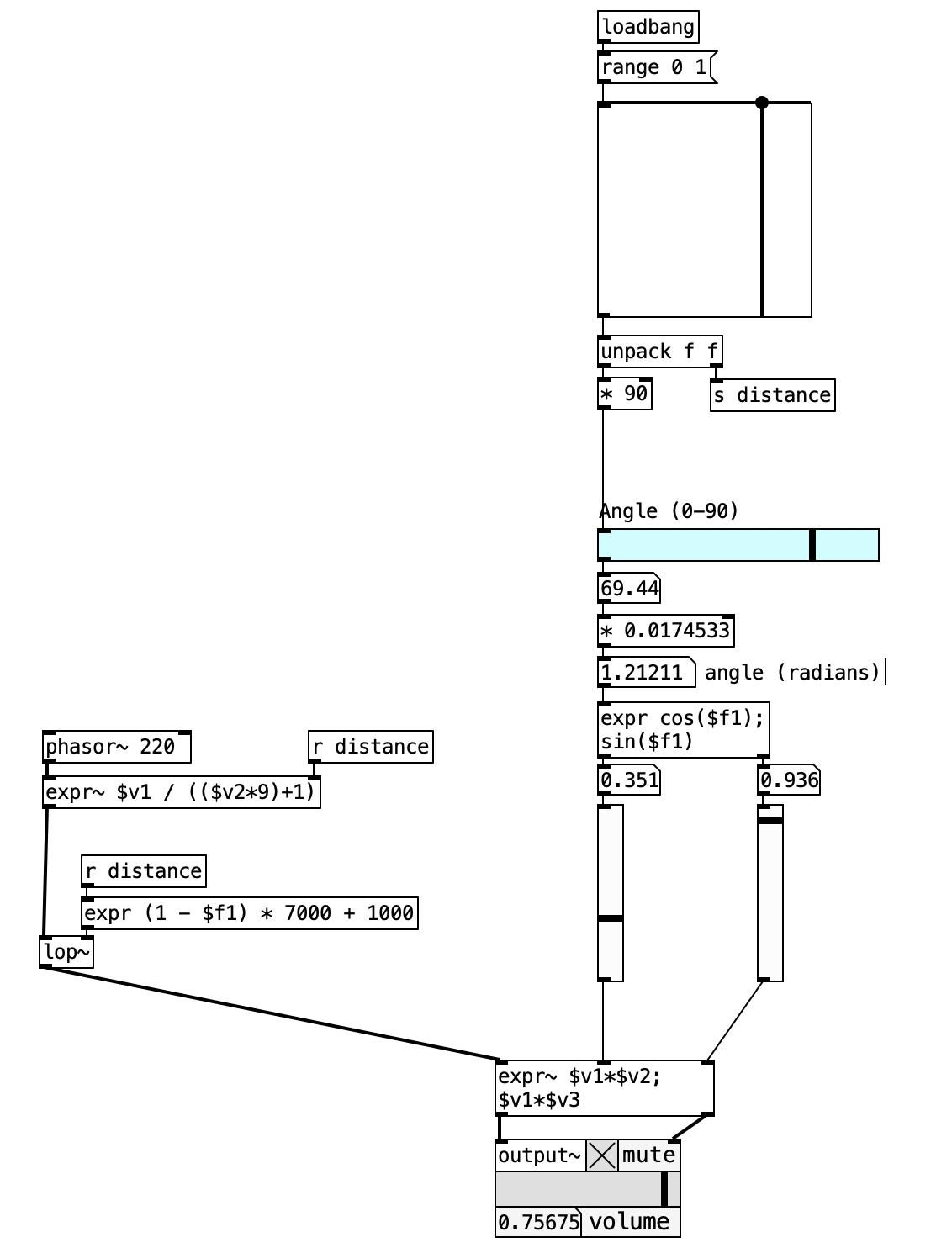
We control the cutoff frequency of this filter using a [expr] object ([expr (1 - $f1) * 7000 + 1000]). For example, we can scale a distance range of 1–10 to a cutoff frequency range of 8000–1000 Hz. As the source moves farther away, the filter reduces the brightness of the sound, mimicking atmospheric filtering.

Consider a large environment with significant reverberation—such as a church or garage. When someone speaks nearby, the direct sound dominates, and reverberation is minimal. Conversely, at greater distances, the direct signal weakens while reverberation remains relatively constant. This is due to the fact that reverberation is a function of the environment and not as sensitive to the source’s location.

Enhanced distance modeling combining amplitude attenuation, low-pass filtering, and dynamic reverberation balance.

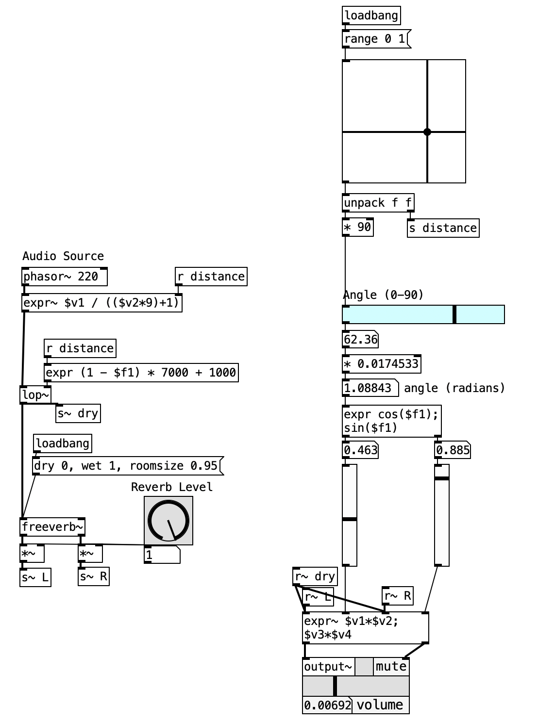
To simulate this phenomenon, we introduce a reverberation chamber using [freeverb~]. The reverb level is controlled via a rotary dial ([knob] from the ELSE library). By configuring the knob for a low initial setting, we simulate the acoustic behavior where reverberation becomes more prominent as the source moves farther from the listener. As the source approaches, the increased amplitude of the direct signal masks the reverberation, completing our auditory illusion.

The patch extends the interactive distance panning system by incorporating realistic acoustic phenomena that occur in natural environments. The implementation adds frequency-dependent air absorption through low-pass filtering and environmental reverberation modeling, creating a comprehensive spatial audio simulation that mirrors how sound behaves across varying distances in real acoustic spaces. This enhanced system demonstrates how multiple acoustic cues work together to create convincing depth perception and environmental context.

The design integrates three primary acoustic distance cues: amplitude attenuation based on inverse distance relationships, high-frequency absorption that simulates atmospheric filtering, and reverberation balance that reflects how direct and reflected sound components change with source proximity. This multi-parameter approach creates significantly more realistic distance simulation than amplitude scaling alone.

6.7.1 Patch Overview

The enhanced distance modeling system implements a comprehensive acoustic simulation pipeline consisting of six integrated processing stages:

1. Two-Dimensional Interface Control: Visual manipulation of angle and distance parameters
2. Distance-Based Amplitude Scaling: Inverse relationship modeling for realistic volume attenuation
3. Frequency-Dependent Air Absorption: Low-pass filtering that simulates atmospheric effects
4. Environmental Reverberation Processing: Spatial acoustic context through algorithmic reverb
5. Direct/Reverb Signal Balancing: Dynamic mixing based on distance relationships
6. Spatial Audio Output: Final stereo positioning with enhanced depth cues

The system demonstrates how multiple acoustic phenomena combine to create convincing spatial audio environments that extend beyond simple amplitude panning.

6.7.1.1 Critical Enhancement Components

Air Absorption Modeling: The lop~ object implements frequency-dependent attenuation that simulates how air absorption affects sound transmission over distance. The cutoff frequency calculation (1 - $f1) * 7000 + 1000 creates an inverse relationship where increased distance produces lower cutoff frequencies, mimicking the natural tendency for high frequencies to attenuate more rapidly through atmospheric transmission.

Reverberation Processing: The freeverb~ object provides environmental acoustic context through algorithmic reverberation that simulates room acoustics. The reverb parameters (dry 0, wet 1, roomsize 0.95) create a large virtual space with minimal direct signal bleed-through.

Dynamic Signal Routing: The send/receive system (s~ dry, r~ dry) enables parallel processing where the same audio source feeds both the direct signal path and the reverberation processing chain, allowing independent control of each component.

6.7.2 Data Flow

flowchart TD
    A[2D Slider Interface] --> B[Distance Extraction]
    B --> C[Amplitude Scaling]
    B --> D[Air Absorption Filtering]
    B --> E[Reverb Level Control]
    F[Audio Source] --> C
    C --> G[Low-pass Filter]
    D --> G
    G --> H[Dry Signal Path]
    G --> I[Reverb Processing]
    E --> I
    H --> J[Spatial Mixing]
    I --> J
    J --> K[Enhanced Stereo Output]
    
    style A fill:#e1f5fe
    style K fill:#f3e5f5
    style G fill:#fff3e0
    style I fill:#fff3e0

The enhanced distance modeling patch orchestrates a sophisticated multi-stage acoustic simulation that combines amplitude, frequency, and temporal cues to create realistic spatial audio experiences. This implementation demonstrates how multiple acoustic phenomena interact in natural environments and how these relationships can be modeled systematically to achieve convincing distance perception.

The enhanced distance parameter extraction stage builds upon the basic distance panning system by distributing the distance control signal to multiple processing destinations simultaneously. The y-coordinate from the 2D slider interface continues to provide the primary distance measurement, but this value now feeds three distinct processing pathways rather than a single amplitude control. The distance parameter reaches the amplitude scaling system for volume attenuation, the air absorption calculation system for frequency filtering, and the reverberation balance system for environmental processing. This parallel distribution ensures that all acoustic distance cues remain synchronized and proportional, maintaining the physical relationships that exist in natural acoustic environments.

The frequency-dependent air absorption processing stage introduces realistic high-frequency attenuation that simulates atmospheric filtering effects. The distance value undergoes transformation through the expression (1 - $f1) * 7000 + 1000, which creates an inverse relationship mapping distance to low-pass filter cutoff frequency. When the source appears close (distance near 0), the calculation yields a cutoff frequency approaching 8000 Hz, allowing the full frequency spectrum to pass through unaffected. As distance increases toward maximum (distance near 1), the cutoff frequency approaches 1000 Hz, creating significant high-frequency attenuation that simulates the natural absorption characteristics of air transmission. The lop~ object implements this filtering in real-time, processing the distance-scaled audio signal to create the spectral changes associated with increasing source distance. This filtering effect proves particularly noticeable with broad-spectrum audio sources, where the gradual loss of high-frequency content creates immediate perceptual cues about source proximity.

The environmental reverberation processing stage adds spatial acoustic context through sophisticated algorithmic processing that simulates how direct and reflected sound components change with source distance. The audio signal enters the freeverb~ object configured with parameters that create a large virtual acoustic space: dry level set to 0 eliminates direct signal bleed-through, wet level at 1 provides full reverberation output, and room size at 0.95 creates an expansive virtual environment. The reverberation level control through the knob interface enables real-time adjustment of the environmental contribution, simulating how reverberation prominence changes with source distance. In natural acoustic environments, nearby sources produce strong direct signals that mask reverberation, while distant sources generate weaker direct signals that allow reverberation to become more prominent in the overall acoustic balance.

The signal mixing and spatial integration stage combines the processed direct and reverberated audio components while maintaining the established spatial positioning relationships. The direct signal path carries the distance-attenuated and air-absorption-filtered audio through the send/receive system (s~ dry, r~ dry) to the spatial mixing stage, while the reverberation output provides environmental context that adds spatial depth and acoustic realism. The final spatial audio expression expr~ $v1*$v2 \; $v3*$v4 applies the trigonometric amplitude coefficients to both the direct and environmental signal components, ensuring that the spatial positioning affects all aspects of the audio output. This integrated approach creates stereo output where both the direct sound and its environmental reflections maintain proper spatial relationships, contributing to convincing three-dimensional audio positioning that extends beyond simple left-right panning.

flowchart LR
    A[Distance Control] --> B[Multi-Parameter Processing]
    B --> C[Enhanced Audio Output]

6.7.3 Processing Chain Details

The enhanced distance modeling system integrates multiple acoustic simulation stages:

Stage	Input	Process	Output
1	2D Interface	Distance parameter extraction	Control signals for multiple destinations
2	Distance Value	Amplitude scaling calculation	Volume attenuation
3	Distance Value	Air absorption frequency mapping	Low-pass filter cutoff
4	Filtered Audio	Environmental reverberation	Spatial acoustic context
5	Distance Value	Reverb balance calculation	Direct/reverb mixing ratio
6	Multiple Audio Streams	Spatial positioning integration	Enhanced stereo output

6.7.3.1 Acoustic Parameter Relationships

Distance Setting	Amplitude	Cutoff Frequency	Reverb Prominence	Perceived Effect
0.0 (Close)	1.000	8000 Hz	Low	Bright, direct, intimate
0.25	0.692	6250 Hz	Low-Medium	Slightly muffled, present
0.5	0.444	4500 Hz	Medium	Noticeably filtered, balanced
0.75	0.308	2750 Hz	Medium-High	Distant, reverberant
1.0 (Far)	0.200	1000 Hz	High	Very distant, heavily filtered

6.7.3.2 Air Absorption Simulation

The frequency mapping implements realistic atmospheric absorption characteristics:

• Near field (0-0.3): Minimal high-frequency loss, preserving audio brightness
• Mid field (0.3-0.7): Progressive filtering that maintains intelligibility
• Far field (0.7-1.0): Significant high-frequency attenuation creating distant character

6.7.4 Key Objects and Their Roles

Object	Function	Role in Enhanced Distance Modeling
slider2d	Two-dimensional interface	Angle and distance parameter input
expr~ $v1 / (($v2*9)+1)	Distance amplitude scaling	Inverse distance attenuation
lop~	Low-pass filter	Frequency-dependent air absorption simulation
expr (1 - $f1) * 7000 + 1000	Cutoff frequency calculation	Maps distance to absorption characteristics
freeverb~	Algorithmic reverberation	Environmental acoustic simulation
s~ dry / r~ dry	Dry signal routing	Direct sound path management
expr~ $v1*$v2 \; $v3*$v4	Spatial audio multiplier	Final stereo positioning with distance effects

6.7.5 Creative Applications

• Cinematic Soundscape Design: Create realistic environmental audio where sound sources exhibit authentic distance characteristics for film, gaming, or virtual reality applications.
• Architectural Acoustic Simulation: Model specific room types by adjusting reverberation parameters to match different environmental contexts from intimate chambers to vast cathedrals.
• Interactive Audio Installations: Design responsive environments where visitor movement controls not just positioning but the complete acoustic experience including filtering and reverberation.
• Nature Sound Recreation: Simulate outdoor acoustic environments where wildlife calls, weather sounds, and ambient textures exhibit realistic distance-dependent characteristics.
• Performance Audio Processing: Process live instruments with dynamic distance effects that can be controlled by performers or automated through score-following systems.

6.8 Simulation through Quadraphonic Spatialization: The Chowning Model

To extend spatial simulation beyond the limitations of stereophony—typically constrained to a 90° field—or to achieve finer localization resolution, the intensity panning technique used with two loudspeakers can be generalized to multi-channel systems.

Chowning quadraphonic spatialization model with lookup table generation, circular interface control, and four-speaker amplitude distribution for 360-degree spatial audio positioning.

By placing four loudspeakers at the corners of a square, one can simulate a 360° horizontal sound field, allowing for a full circular distribution of a virtual source. Arranging six speakers in a hexagonal layout also provides 360° coverage, with improved localization accuracy. As a general rule, more channels yield higher resolution and spatial definition, though this comes at the cost of increased system complexity. From a practical standpoint, quadraphonic configurations have proven to offer a compelling balance between implementation feasibility and perceptual quality, and have thus gained wide acceptance in spatial sound simulation.

One of the most well-known models in this domain is the John Chowning quadraphonic model. It features:

• Direct sound simulation from a virtual source
• Local reverberation, individually tailored for each speaker based on the source’s angle
• Global reverberation shared across all four speakers

6.8.1 Amplitude and Distance Scaling

The audio input signal is first attenuated according to the inverse of the distance:

\[ A_{\text{direct}} = \frac{1}{D} \]

Then, the signal is scaled by a coefficient specific to each speaker, depending on the virtual source’s position:

\[ A_i = \frac{1}{D} \times C_i(\theta) \]

where:

• \(A_i\) is the amplitude for speaker \(i\),
• \(D\) is the distance between the source and the listener,
• \(C_i(\theta)\) is the coefficient for speaker \(i\) as a function of the source angle \(\theta \in [0^\circ, 360^\circ]\),
• and the speaker coefficients are labeled LRA, LFA, RFA, RRA (Left Rear, Left Front, Right Front, Right Rear).

6.8.2 Gain Function and Phase Offsets

To avoid complex calculations of gain for each speaker, Chowning implements a predefined function, stored as a lookup table of 512 samples. The table’s function ranges between 0 and 1 and is designed to generate continuous 360° source motion through intensity panning.

Each speaker reads the same function with a phase offset:

• The first quarter of the function represents a sine wave from \(0^\circ\) to \(90^\circ\)
• The second quarter is a cosine wave over the same angular range
• The remaining half is silent (zero amplitude)

As the virtual source rotates, only two speakers are active at a time, crossfading between them. For instance, as the source moves from \(theta = 90^\circ\) to \(\theta = 0^\circ\), the cosine-driven speaker fades out while the sine-driven speaker fades in, mimicking a continuous spatial trajectory.

6.8.3 Reverberation Modeling

In the lower part of Chowning’s model (see again Figure G.8.9), reverberation is processed separately: - The reverberation signal is attenuated by the square root of the inverse of the distance:

\[ A_{\text{reverb}} = \sqrt{\frac{1}{D}} \times \text{PRV} \]

where PRV is an empirical parameter representing the reverberation percentage.

• A global reverb signal is scaled again by \(\frac{1}{D}\)
• Local reverberation is further attenuated by \(1 - \frac{1}{D}\), then scaled using the same angle-dependent coefficients (LRA, LFA, RFA, RRA)

To increase realism, four independent reverberation units are used—one for each loudspeaker—ensuring spatial decorrelation and more convincing immersion.

This model not only exemplifies how mathematical reasoning and spatial design converge in sound synthesis, but also stands as a landmark in algorithmic composition and immersive audio. Through relatively simple mathematical operations and efficient data structures (such as phase-offset lookup tables), it offers a powerful foundation for dynamic spatial control in real-time systems such as Pd.

6.8.4 Coordinate System

The circle object gives you Cartesian coordinates (x, y) in range [-1, 1], but you need:

1. Polar coordinates (angle, radius)
2. Scaled values (0-359° for azimuth, 1-10 for distance)

6.8.5 Mathematical Conversion

6.8.5.1 Azimuth (Angle) Calculation

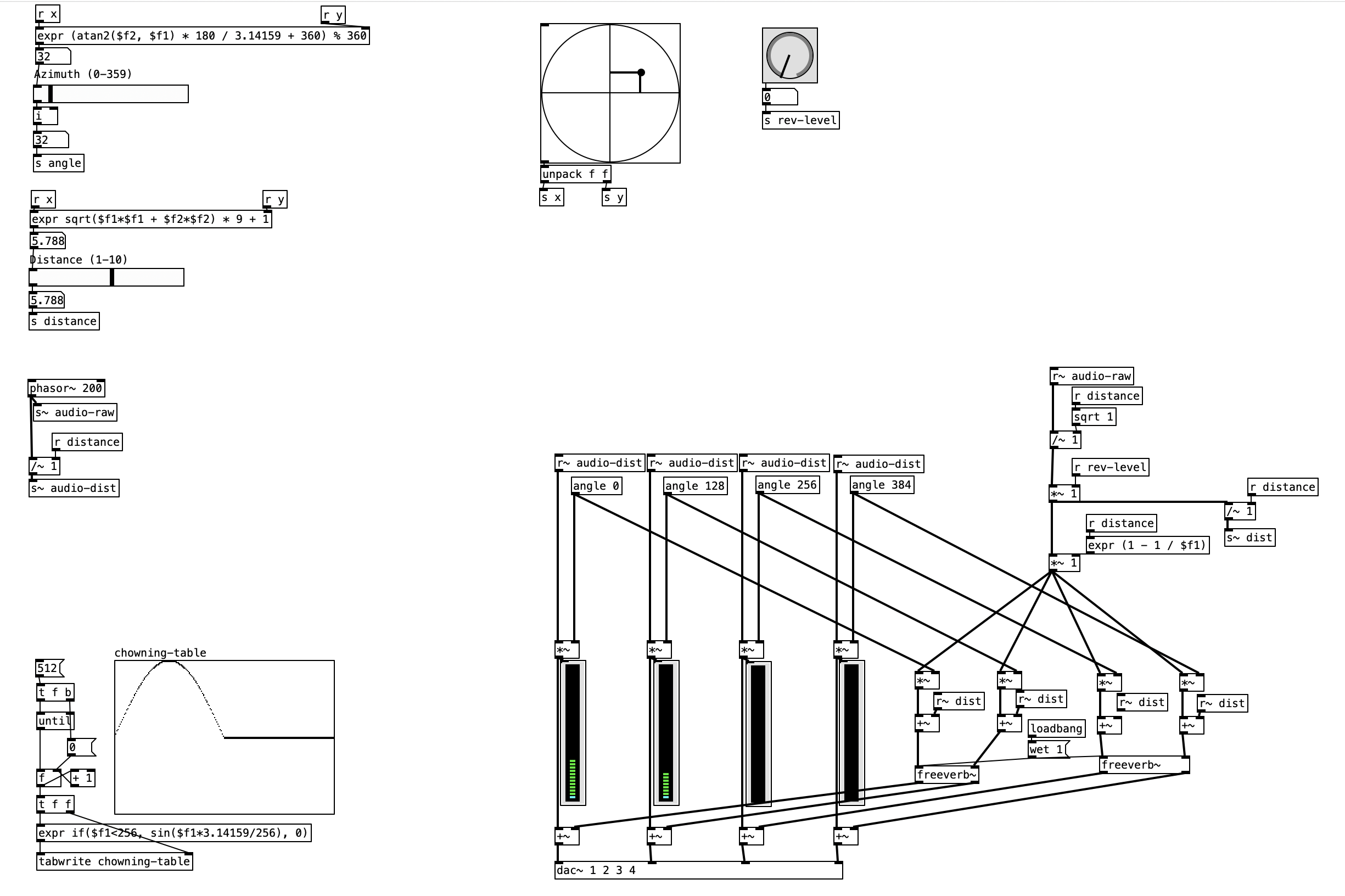
We need to convert (x, y) to angle using arctangent using:

[expr atan2($f2, $f1) * 180 / 3.14159]

Key points:

• atan2(y, x) gives angle in radians (-π to π)
• Multiply by 180/π to convert to degrees (-180° to 180°)
• Add 360° if negative to get 0-360° range:

[expr (atan2($f2, $f1) * 180 / 3.14159 + 360) % 360]

6.8.5.2 Distance Calculation

Convert (x, y) to radius using Pythagorean theorem, then scale:

[expr sqrt($f1*$f1 + $f2*$f2) * 9 + 1]

Logic:

• sqrt(x² + y²) gives radius in range [0, 1]
• Multiply by 9 and add 1 to get range [1, 10]

6.8.6 Patch Overview

This Pd patch implements John Chowning’s groundbreaking quadraphonic spatialization model, demonstrating how mathematical algorithms can create convincing 360-degree spatial audio movement using four strategically positioned speakers. The implementation features a predefined lookup table, distance-based amplitude scaling, and sophisticated reverberation modeling that simulates both local and global acoustic environments. This approach enables precise control over virtual sound source movement while maintaining perceptual coherence across the complete circular sound field.

The patch demonstrates the practical application of Chowning’s theoretical framework through real-time interface controls that manage azimuth positioning, distance simulation, and reverberation balance. By utilizing lookup tables and phase-offset techniques, the system achieves smooth spatial transitions while minimizing computational overhead, making it suitable for live performance and interactive applications.

The Chowning quadraphonic spatialization system implements a comprehensive spatial audio pipeline consisting of six primary processing stages:

1. Lookup Table Generation: Creates the fundamental sine/cosine function for spatial positioning
2. Interactive Control Interface: Manages azimuth, distance, and reverberation parameters
3. Amplitude Coefficient Calculation: Determines speaker-specific gain values using phase offsets
4. Distance Modeling: Applies inverse distance relationships for realistic amplitude scaling
5. Reverberation Processing: Implements both local and global acoustic environment simulation
6. Quadraphonic Output: Delivers positioned audio to four independent speaker channels

The system demonstrates how relatively simple mathematical operations and efficient data structures can create sophisticated spatial audio experiences suitable for both compositional and performance applications.

6.8.6.1 Critical Processing Components

Chowning Lookup Table: The 512-sample array contains a complete sine function from 0° to 180° (samples 0-255) followed by silence (samples 256-511). This creates the characteristic amplitude envelope where only two adjacent speakers are active at any time during 360° rotation.

Angle Objects: Each of the four speakers uses an angle object with specific phase offsets (0, 128, 256, 384) that correspond to 90° increments around the circular speaker arrangement. These offsets ensure proper spatial positioning as the virtual source rotates.

Dynamic Distance Processing: The patch implements both amplitude attenuation (/~ distance) and reverberation balance modification (sqrt and 1-1/distance calculations) to create realistic distance perception through multiple acoustic cues.

6.8.7 Data Flow

flowchart TD
    A[Lookup Table Generation] --> B[Interface Controls]
    B --> C[Amplitude Calculation]
    B --> D[Distance Processing]
    C --> E[Audio Positioning]
    D --> E
    E --> F[Reverberation]
    F --> G[Quadraphonic Output LF RF RR LR]
    
    style A fill:#e1f5fe
    style G fill:#f3e5f5
    style E fill:#fff3e0
    style F fill:#fff3e0

The Chowning quadraphonic spatialization patch orchestrates a sophisticated multi-stage spatial audio processing pipeline that transforms user interface input into convincing 360-degree sound source positioning through mathematical modeling of acoustic propagation and psychoacoustic principles. This implementation demonstrates how John Chowning’s theoretical framework translates into practical real-time audio processing systems that maintain both computational efficiency and perceptual accuracy.

The lookup table generation and initialization stage establishes the mathematical foundation for the entire spatialization system through automated creation of the characteristic Chowning function. Upon patch initialization, the loadbang object triggers a systematic process that populates the chowning-table array with 512 samples representing the fundamental spatial positioning function. The generation process employs an until loop that iterates through array indices 0-511, with each position calculated using the expression if($f1<256, sin($f1*3.14159/256), 0). This creates a complete sine wave from 0° to 180° occupying the first half of the table (samples 0-255), followed by complete silence in the second half (samples 256-511). This specific function design ensures that during 360° spatial rotation, only two adjacent speakers remain active at any time, creating smooth amplitude transitions that maintain constant energy output while avoiding phase cancellation effects that could degrade spatial imaging.

The interactive control and parameter extraction stage manages real-time spatial positioning through the sophisticated interface provided by the circle object from the ELSE library. This two-dimensional control surface captures mouse interaction as normalized coordinate pairs that represent both angular position and distance information within a single intuitive interface. The coordinate unpacking process separates the combined spatial input into independent data streams: the x-coordinate undergoes conversion to azimuth values spanning 0-359° through the expression (atan2($f2, $f1) * 180 / 3.14159 + 360) % 360, while the y-coordinate transforms into distance values ranging 1-10 through sqrt($f1*$f1 + $f2*$f2) * 9 + 1. This dual parameter extraction enables simultaneous control over both horizontal positioning and depth perception within the virtual acoustic space, providing the essential control data for subsequent processing stages.

The amplitude coefficient calculation stage represents the core of Chowning’s spatialization algorithm, where angular position information becomes speaker-specific gain values through phase-offset table reading. Each of the four speakers employs an individual angle object configured with specific phase offsets: 0 samples for the front-left speaker, 128 samples for front-right, 256 samples for rear-right, and 384 samples for rear-left. These offsets correspond to 90° increments around the circular speaker arrangement, ensuring that the spatial positioning function provides appropriate amplitude coefficients for each speaker location. As the azimuth value changes, each angle object reads from its phase-shifted position within the lookup table, generating amplitude coefficients that create smooth transitions between adjacent speakers while maintaining the characteristic two-speaker activation pattern that defines the Chowning model.

The distance processing and amplitude scaling stage implements realistic sound propagation characteristics through multiple coordinated processing pathways that simulate both amplitude attenuation and acoustic environmental effects. The primary distance attenuation employs the expression expr~ $v1 / (($v2*9)+1) applied to the raw audio signal, creating inverse distance scaling where increasing distance produces proportionally decreased amplitude. This amplitude scaling affects all speakers equally, maintaining the spatial positioning relationships while adding realistic volume changes that correspond to source proximity. Simultaneously, the distance parameter influences reverberation processing through the sqrt calculation that modifies reverberation level based on distance relationships, simulating how nearby sources produce strong direct signals that mask environmental reflections while distant sources allow reverberation to become more prominent in the overall acoustic balance.

The reverberation processing and environmental simulation stage adds spatial acoustic context through dual-path processing that creates both local and global environmental effects. The audio signal path splits to feed both direct positioning processing and environmental reverberation systems implemented through freeverb~ objects configured for large virtual spaces. The reverberation balance control through the knob interface enables real-time adjustment of environmental contribution, while the distance-dependent reverberation scaling creates realistic acoustic behavior where reverberation prominence varies with source distance. The dual reverberation system provides both general environmental ambience and speaker-specific local reflections, creating convincing spatial acoustic contexts that enhance the positioning effects achieved through the amplitude coefficients.

flowchart LR
    A[User Input] --> B[Parameter Processing]
    B --> C[Spatial Calculation]
    C --> D[Audio Output]

6.8.8 Processing Chain Details

The quadraphonic spatialization system maintains mathematical precision and perceptual coherence through coordinated processing stages:

Stage	Input	Process	Output
1	Patch Initialization	Sine function generation	512-sample lookup table
2	Circle Interface	Coordinate conversion	Azimuth (0-359°) and Distance (1-10)
3	Azimuth + Phase Offsets	Table reading with interpolation	Speaker amplitude coefficients
4	Distance Value	Inverse scaling calculation	Amplitude attenuation factor
5	Audio + Coefficients + Distance	Multiplication and mixing	Positioned audio signals
6	Multiple Audio Streams	Reverberation processing	Enhanced quadraphonic output

6.8.8.1 Speaker Configuration and Phase Offsets

Speaker Position	Phase Offset (samples)	Angle Equivalent	Function Region
Front Left (LF)	0	0°	Sine ascending
Front Right (RF)	128	90°	Sine descending
Rear Right (RR)	256	180°	Silent region
Rear Left (LR)	384	270°	Silent region

6.8.8.2 Distance Processing Parameters

Distance Value	Amplitude Scaling	Reverberation Factor	Perceived Effect
1.0 (Close)	1.000	0.000	Immediate, dry, present
3.0	0.250	0.667	Moderate distance, some reverb
6.0	0.143	0.833	Distant, reverberant
10.0 (Far)	0.091	0.900	Very distant, highly reverberant

6.8.8.3 Lookup Table Function Analysis

The Chowning table implements a specific mathematical relationship that ensures smooth spatial transitions:

• Samples 0-127: Ascending sine (0 to 1) - Controls fade-in transitions
• Samples 128-255: Descending sine (1 to 0) - Controls fade-out transitions
  
• Samples 256-511: Silent (0) - Ensures two-speaker limitation

This function design creates the characteristic “phantom source” effect where virtual positioning occurs between active speaker pairs while maintaining constant total energy output.

6.8.9 Key Objects and Their Roles

Object	Function	Role in Quadraphonic System
tabwrite chowning-table	Lookup table creation	Stores 512-sample sine function for spatial coefficients
expr if($f1<256, sin($f1*3.14159/256), 0)	Function generation	Creates sine wave with silent half-cycle
circle	2D position interface	Provides x,y coordinates for azimuth and distance control
angle	Phase offset calculation	Implements speaker-specific table reading positions
freeverb~	Algorithmic reverberation	Creates environmental acoustic simulation
expr~ $v1 / (($v2*9)+1)	Distance attenuation	Applies inverse distance amplitude scaling
sqrt	Reverberation scaling	Modifies reverb balance based on distance

6.8.10 Creative Applications

• 360-Degree Spatial Composition: Create immersive musical pieces where sound sources move in complete circles around the listener, utilizing the full quadraphonic field for dynamic spatial narratives.
• Interactive Spatial Performance: Connect external controllers or sensors to the azimuth and distance parameters, enabling performers to sculpt spatial positioning through gesture or movement.
• Environmental Sound Design: Simulate realistic acoustic environments by combining the Chowning positioning with distance-dependent reverberation for film, game, or installation applications.
• Multi-Source Spatial Mixing: Implement multiple instances of the Chowning model to position independent sound sources within the same quadraphonic field, creating complex spatial polyphony.
• Adaptive Concert Hall Simulation: Use real-time reverberation control to simulate different acoustic environments during performance, from intimate chambers to vast cathedrals.
• Collaborative Virtual Environments: Network multiple quadraphonic systems where remote participants can position sounds within shared virtual acoustic spaces for telepresence applications.

6.9 Mid/Side (M/S) Processing

Mid/Side (M/S) processing is a stereo audio technique that transforms conventional left/right stereo signals into a representation consisting of mid (center) and side (stereo difference) components. This transformation enables precise independent manipulation of the central mono-compatible content and the peripheral stereo information, providing powerful creative control over stereo imaging and spatial characteristics. The technique finds extensive application in mixing, mastering, and sound design contexts where selective processing of spatial components is required.

The M/S approach offers unique advantages over conventional stereo processing by separating spatial information into functionally distinct components. The mid channel contains the sum of left and right signals, representing content that appears centered in the stereo field, while the side channel contains the difference between left and right signals, representing the spatial width and ambience information. This separation enables processing strategies that would be impossible with conventional L/R stereo signals.

Mid/side stereo processing with adjustable “width” control.

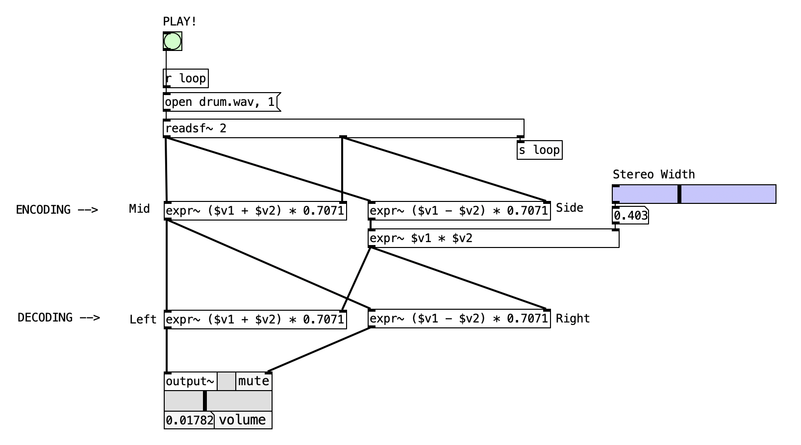
6.9.1 Historical Context

The Mid/Side (M/S) microphone recording technique is not a recent innovation. It was originally conceived by Alan Blumlein, a British engineer working at EMI and a pivotal figure in the development of stereophonic and surround sound. Blumlein patented the M/S technique in 1933, and it was implemented in some of the earliest stereophonic recordings, laying the foundation for much of what would follow in multichannel audio. Over time, M/S recording has found widespread adoption in broadcasting due to its inherent mono compatibility—a critical requirement in transmission environments where listeners may receive a downmixed signal. Its adaptability has also made it a mainstay in studio environments, where precise control over stereo width is valued, as well as in live recording scenarios, where on-site flexibility is essential.

6.9.2 Why Choose Mid/Side?

One of the key advantages of M/S over traditional XY stereo techniques lies in its post-production flexibility. In XY configurations, the stereo image is fixed at the moment of recording. Any adjustments to the spatial field must be made prior to—or during—recording, leaving limited room for change afterward. Additionally, summing XY recordings to mono can result in undesirable phase cancellations, compromising audio quality.

In contrast, the M/S technique allows for the stereo width to be manipulated even after the recording session. By adjusting the balance between the mid and side signals, engineers can widen, narrow, or even collapse the stereo image to mono without destructive artifacts. This makes M/S a powerful tool for both artistic control and technical resilience.

MS recording technique: The Mid mic acts as the center channel, while the Side mic signal creates the stereo ambience.

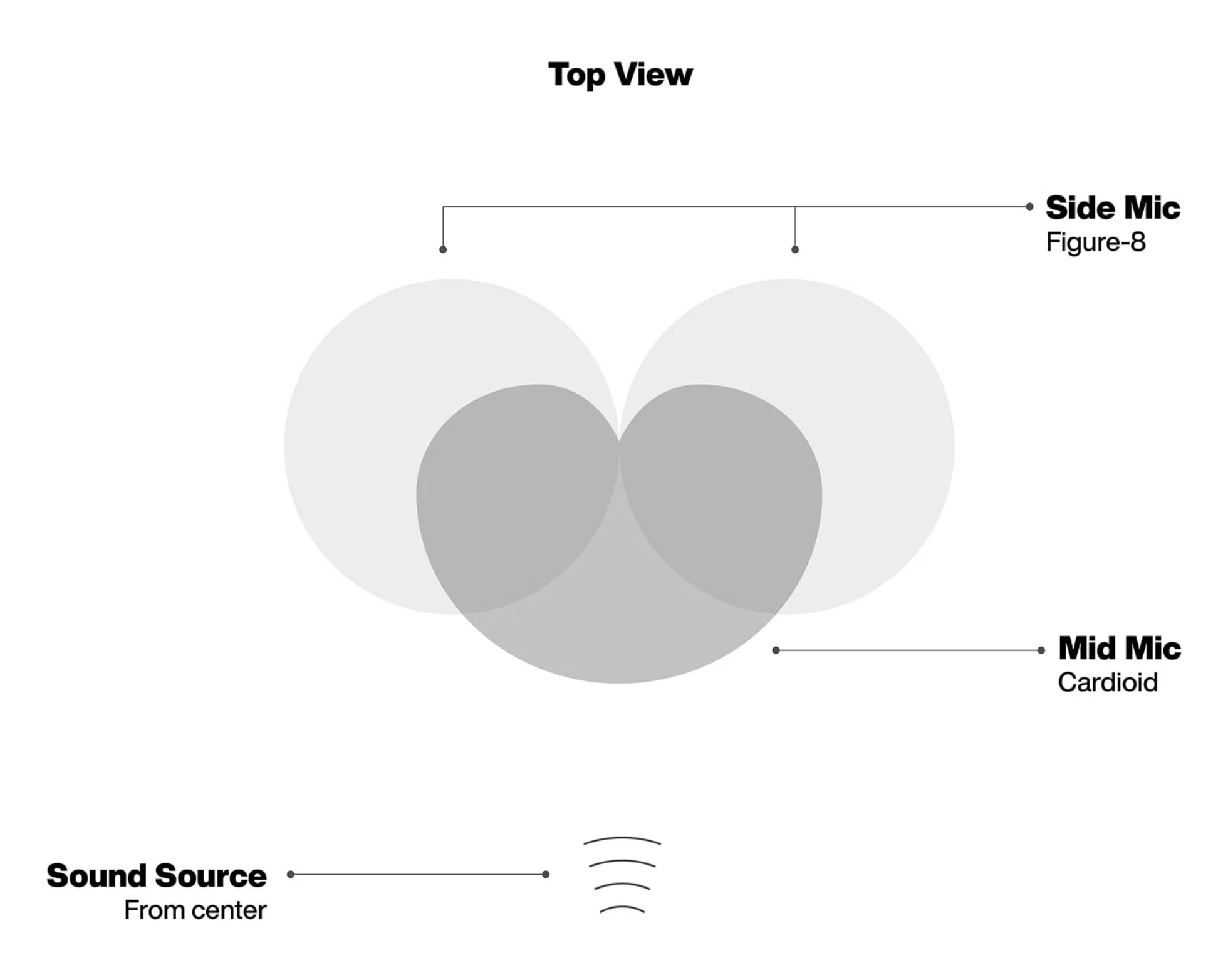
The core concept of M/S recording is elegantly simple yet powerful. The Mid microphone captures the central, on-axis sound—essentially forming the mono-compatible core of the stereo image. The Side microphone, with its figure-8 pattern, captures ambient and directional information from either side of the soundstage.

The critical feature of the Side mic is that its two lobes are 180 degrees out of phase. This means that a pressure increase on one side of the diaphragm results in an equivalent pressure decrease on the other. Conventionally, the positive lobe (+) is oriented to the left, while the negative lobe (−) faces the right side of the soundstage. When decoded into stereo, this phase relationship creates lateral cues that define the width and spatial depth of the stereo field.

6.9.3 Patch Overview

The mid-side-stereo.pd patch implements a complete M/S processing system that demonstrates both encoding and decoding stages within a single interface. The patch features a stereo audio file player (drum.wav) that feeds into an M/S encoder, followed by a stereo width control that manipulates the side channel amplitude, and finally an M/S decoder that reconstructs the stereo signal. This architecture enables real-time demonstration of how M/S processing affects stereo imaging while maintaining mathematical precision throughout the signal chain.

The system incorporates a sophisticated stereo width control mechanism that allows users to adjust the prominence of the side channel from complete mono (width = 0) to exaggerated stereo enhancement (width > 1). This control provides immediate auditory feedback about how M/S processing affects spatial perception while demonstrating the mathematical relationships underlying stereo imaging manipulation.

The patch design emphasizes educational clarity by implementing the encoding and decoding stages as separate processing blocks with clear signal flow visualization. The mathematical operations are implemented using expr~ objects that execute the precise calculations required for M/S transformation while maintaining the amplitude relationships essential for accurate stereo reconstruction.

6.9.4 Data Flow

flowchart TD
    A[Audio File Player] --> B[Stereo Input L/R]
    B --> C[M/S Encoding]
    C --> D[Mid Channel M = L + R]
    C --> E[Side Channel S = L - R]
    E --> F[Stereo Width Control]
    F --> G[Modified Side Channel]
    D --> H[M/S Decoding]
    G --> H
    H --> I[Left Output L = M + S * 0.7071]
    H --> J[Right Output R = M - S * 0.7071]
    I --> K[Stereo Audio Output]
    J --> K
    
    style A fill:#e1f5fe
    style K fill:#f3e5f5
    style C fill:#fff3e0
    style H fill:#fff3e0

The M/S processing patch orchestrates a comprehensive stereo transformation pipeline that demonstrates both the mathematical principles and practical applications of mid/side processing through systematic signal manipulation stages. This implementation provides real-time control over stereo imaging while maintaining the mathematical relationships essential for accurate audio reconstruction.

The audio source and initialization stage establishes the foundation for M/S processing through automated stereo audio file playback that provides consistent source material for demonstration purposes. The readsf~ 2 object loads and plays the stereo audio file drum.wav, providing left and right channel audio streams that serve as input to the M/S processing chain. The looping mechanism implemented through the bang connection from the third outlet of readsf~ to the s loop send object ensures continuous playback that enables sustained observation of the M/S processing effects. The manual playback control through the PLAY! button provides user initiation of the audio source, while the file opening message open drum.wav, 1 prepares the stereo audio file for processing. This source material selection proves particularly effective for M/S demonstration because drum recordings typically contain both centered elements (kick, snare) that appear prominently in the mid channel and peripheral elements (cymbals, room ambience) that contribute significantly to the side channel.

The M/S encoding stage implements the fundamental mathematical transformation that separates stereo spatial information into functionally distinct mid and side components through parallel expression processing. The stereo input from the audio file feeds into two separate expr~ objects that perform the essential M/S calculations: the mid channel calculation through expr~ ($v1 + $v2) * 0.7071 creates the sum of left and right channels with appropriate amplitude scaling, while the side channel calculation through expr~ ($v1 - $v2) * 0.7071 generates the difference between left and right channels similarly scaled. The scaling factor 0.7071 (1/√2) ensures proper amplitude relationships that prevent signal overflow while maintaining mathematical accuracy throughout the encoding process. This encoding stage transforms the conventional stereo signal into a representation where the mid channel contains all centered audio content and the side channel contains all spatial width information, enabling independent manipulation of these components.

The stereo width control and side channel modification stage provides real-time manipulation of the spatial characteristics through user interface control that affects the prominence of the side channel information. The horizontal slider (hsl) interface element provides intuitive control over stereo width, with values ranging from 0 (complete mono) to 1 (original stereo width) and beyond for enhanced stereo effects. The slider output connects to a float atom display that provides numerical feedback of the current width setting, enabling precise control over the spatial manipulation amount. The width control value feeds into the expr~ $v1 * $v2 expression that multiplies the side channel signal by the user-controlled width factor, directly affecting how much spatial information contributes to the final stereo reconstruction. This multiplication approach enables smooth transitions from mono (width = 0, side channel eliminated) through original stereo imaging (width = 1, side channel unaffected) to enhanced stereo width (width > 1, side channel emphasized).

The M/S decoding and stereo reconstruction stage converts the processed mid and side components back into conventional left/right stereo format through mathematical operations that reverse the encoding transformation while incorporating the width modifications. The decoding process employs two expr~ objects that implement the inverse M/S transformation: the left channel reconstruction through expr~ ($v1 + $v2) * 0.7071 combines the mid channel with the width-modified side channel, while the right channel reconstruction through expr~ ($v1 - $v2) * 0.7071 combines the mid channel with the inverted width-modified side channel. These calculations ensure that centered audio content (prominent in the mid channel) appears equally in both output channels while spatial content (contained in the side channel) contributes to the left-right differences that create stereo imaging. The 0.7071 scaling factor applied during decoding maintains proper amplitude relationships and prevents the signal amplification that would otherwise result from the mathematical operations.

The output and monitoring stage delivers the processed stereo audio while providing visual feedback about the processing parameters through integrated display elements that enable users to understand the relationship between control input and audio output characteristics. The final stereo signal feeds into the output~ object that manages audio interface connection and level control for monitoring purposes. The numerical displays connected to various processing stages show the current width parameter value and provide visual indication of the signal processing activity through the connected bang objects. This monitoring system enables users to observe how changes to the stereo width control immediately affect the audio output while providing confirmation that the M/S processing maintains proper signal levels and stereo relationships.

flowchart LR
    A[Stereo Input] --> B[M/S Encode]
    B --> C[Width Control]
    C --> D[M/S Decode]
    D --> E[Stereo Output]

6.9.5 Processing Chain Details

The M/S processing system maintains mathematical precision through coordinated processing stages:

Stage	Input	Process	Output
1	Stereo Audio File	File loading and playback	Left and right audio channels
2	L/R Channels	M/S encoding with scaling	Mid and side channels
3	Side Channel + Width Control	Amplitude multiplication	Modified side channel
4	Mid + Modified Side	M/S decoding with scaling	Reconstructed L/R channels
5	Processed Stereo	Audio interface output	Final stereo audio

6.9.6 Mathematical Relationships

The mathematical foundation of M/S processing is straightforward and relies on simple linear operations.

To encode a standard left/right (L/R) stereo signal into mid and side channels, the following equations are used:

\[ \begin{align*} M &= L + R \\ S &= L - R \end{align*} \]

Here, \((M)\) (mid) represents the sum of the left and right channels, capturing the content that is common to both (centered in the stereo field), while \((S)\) (side) represents the difference, capturing the elements that are unique to each channel (the stereo width).

To decode and return to the conventional stereo format, the inverse operation is performed:

\[ \begin{align*} L &= \frac{M + S}{2} \\ R &= \frac{M - S}{2} \end{align*} \]

The division by 2 in the decoding equations is crucial. Without this scaling, the amplitude of the reconstructed left and right channels would be doubled, potentially causing clipping or an unnatural increase in loudness. This scaling ensures that the energy of the signal remains consistent before and after the M/S transformation.

In practice, instead of dividing by 2, it is common to apply a gain correction of \((-3\,\mathrm{dB})\), which corresponds to multiplying each channel by:

\[ \frac{1}{\sqrt{2}} \approx 0.7071 \]

This factor is used because when both channels are summed or differenced, their combined amplitude could reach up to twice the original value. By scaling each by (0.7071), the total energy is preserved:

\[ 2 \times 0.7071 \times 0.7071 \approx 1 \]

This approach maintains amplitude consistency and prevents distortion, ensuring that a round-trip conversion (L/R \(\rightarrow\) M/S \(\rightarrow\) L/R) yields a signal with the same loudness as the original.

M/S processing is widely used in mixing and mastering. It allows engineers to adjust the stereo width, enhance mono compatibility, or apply effects selectively to the mid or side components. For example, boosting the side channel can widen the stereo image, while attenuating it can make the mix more mono-compatible. Creative sound design often involves processing the mid and side channels differently, such as adding reverb only to the sides or compressing the mid for a punchier center.

A notable feature of M/S processing is its symmetry: the same mathematical structure is used for both encoding and decoding, differing only by the scaling factor. This symmetry arises because the conversion matrix for M/S is its own inverse (up to scaling), which simplifies both implementation and modularity in digital audio environments like Pure Data, Max/MSP, or custom DSP code. This efficiency, combined with its creative flexibility, makes M/S processing a staple in modern audio production.

The patch implements the fundamental M/S transformation equations with proper amplitude scaling:

Parameter	Mathematical Function	Audio Application
Mid Encoding	\(M = (L + R) \times 0.7071\)	Sum channels with amplitude correction
Side Encoding	\(S = (L - R) \times 0.7071\)	Difference channels with amplitude correction
Width Modification	\(S' = S \times W\)	Apply user-controlled width factor
Left Decoding	\(L' = (M + S') \times 0.7071\)	Reconstruct left with processed side
Right Decoding	\(R' = (M - S') \times 0.7071\)	Reconstruct right with processed side

6.9.7 Stereo Width Control Effects

Width Setting	Side Channel Scaling	Stereo Effect	Practical Application
0.0	Complete elimination	Mono (no stereo width)	Mono compatibility checking
0.5	50% reduction	Narrowed stereo image	Subtle width reduction
1.0	Original level	Unchanged stereo width	Bypass/reference setting
1.5	50% enhancement	Widened stereo image	Stereo enhancement
2.0	Double amplitude	Significantly widened	Extreme stereo effects

6.9.8 Key Objects and Their Roles

Object	Function	Role in M/S Processing
readsf~ 2	Stereo file player	Provides consistent stereo source material
expr~ ($v1 + $v2) * 0.7071	Mid channel encoder	Calculates sum of L/R with amplitude scaling
expr~ ($v1 - $v2) * 0.7071	Side channel encoder	Calculates difference of L/R with amplitude scaling
expr~ $v1 * $v2	Width control multiplier	Applies user-controlled scaling to side channel
Width control	Stereo width interface	Provides real-time control over spatial width
output~	Stereo audio output	Delivers processed stereo audio for monitoring

6.9.9 Creative Applications

• Stereo Width Control: Use for dynamic stereo imaging effects in music production, from subtle width adjustments to dramatic spatial effects that respond to musical dynamics or external control sources.

• Mono Compatibility Optimization: Employ during mixing and mastering to check how stereo mixes translate to mono playback systems, ensuring critical elements remain audible when stereo width is eliminated.

• Creative Sound Design: Apply different processing to mid and side channels independently—for example, compress the mid channel for punchy center content while adding reverb only to the side channel for enhanced ambience.

• Live Performance Control: Connect the width parameter to MIDI controllers or OSC input for real-time spatial manipulation during live electronic music performances or DJ sets.

• Mastering Enhancement: Implement as part of mastering chains where precise control over stereo imaging enables correction of mix balance issues or enhancement of spatial characteristics.

• Installation Art: Create responsive audio environments where visitor proximity or movement controls stereo width, creating intimate mono experiences that expand to full stereo as people move through the space.

References

Abregú, E. L., E. R. Calcagno, and R. O. Vergara. 2012. “La Distancia Como Factor Estructural de La Música.” Revista Argentina de Musicología, no. 12-13: 379–400.

Basso, Gustavo, Oscar Pablo Di Liscia, and Juan Pampin, eds. 2009. Música y Espacio: Ciencia, Tecnología y Estética. Buenos Aires: Editorial de la Universidad Nacional de Quilmes.

Knudsen, V. O. 1932. Architectural Acoustics. J. Wiley y Sons.

Risett, J. C. 1969. “An Introductory Catalogue of Computer Synthesized Sounds.” Nueva Jersey: Bell Telephone Laboratories.

Schaeffer, Pierre. 2003. Tratado de Los Objetos Musicales. Translated by Araceli Cabezón de Diego. Alianza Editorial.

Stockhausen, Karlheinz. 1959. “Musik Im Raum.” Die Reihe, no. 5.

Wishart, Trevor. 1996. On Sonic Art. Amsterdam: Harwood Academic Publishers.