2 Sequencing

In this chapter, we will explore the concept of sequencers and how they can be implemented in Pd. We will cover various types of sequencers, including step sequencers, random sequencers, and algorithmic composition techniques, with practical examples and implementations.

2.1 Arrays and Sequencers

Sequencer is a tool for organizing and controlling the playback of events in a temporally ordered sequence. This sequence consists of a series of discrete steps, where each step represents a regular time interval and can contain information about event activation or deactivation. In addition to controlling musical events such as notes, chords, and percussions, a step sequencer can also manage a variety of other events. This includes parameter changes in virtual instruments or audio/video synthesizers, real-time effect automation, lighting control in live performances or multimedia installations, triggering of samples to create patterns and effect sequences, as well as firing MIDI control events to operate external hardware or software. The following table illustrates the basic structure of a step sequencer:

Step	1	2	3	4	5	6	7	8
Value	x	x	x	x	x	x	x	x
Index	0	1	2	3	4	5	6	7

Where:

Each cell represents a step in the sequencer.
1 to 8 indicate the steps.
Empty cells represent steps without events or notes.
You can fill each cell with notes or events to represent the desired sequence.

2.1.1 Formulation (pseudo code)

Data Structures:
- Define a data structure to represent each step of the sequence (e.g., array, list).

Variables:
- Define an array to store the MIDI note values for each step.
- Initialize the sequencer parameters:
  - CurrentStep = 0
  - Tempo
  - NumberOfSteps = 8

Algorithm:
1. Initialization:
   a. Set CurrentStep to 0.
   b. Ask the user to input the Tempo.
   c. Set NumberOfSteps to 8.

2. Loop:
   a. While true:
      i. Calculate the time duration for each step based on the Tempo.
      ii. Play the MIDI note corresponding to the CurrentStep.
      iii. Increment CurrentStep.
      iv. If CurrentStep exceeds NumberOfSteps, reset it to 0.
      v. Wait the calculated duration before moving to the next step.

2.2 Implementation of the 8-Step Sequencer

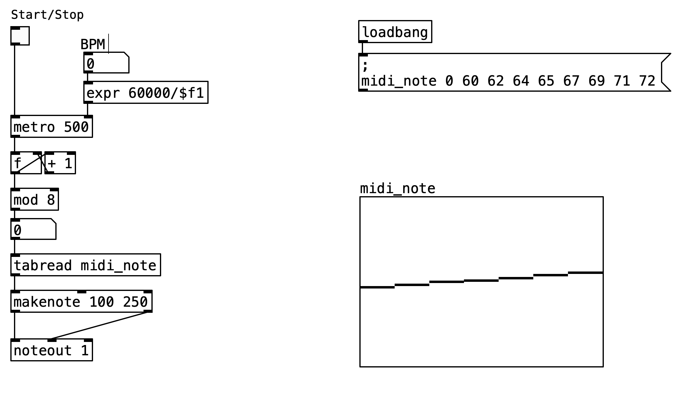
Fig.Implementation of an 8-step MIDI sequencer showing the complete signal flow from tempo control through step counting, array lookup, and MIDI output generation

This implementation demonstrates how to create a basic 8-step MIDI sequencer that cycles through a predefined sequence of notes at a controllable tempo. The patch showcases essential concepts including timing control, array-based data storage, step counting with modulo arithmetic, and MIDI output generation.

2.2.1 Patch Overview

The 8-step sequencer patch implements a classic step-based sequencing paradigm where musical events are organized into discrete time slots. The patch operates by maintaining an internal counter that advances through eight sequential positions, with each position corresponding to a MIDI note value stored in an array. The sequencer provides real-time tempo control through a BPM slider interface and uses Pd’s built-in MIDI capabilities to output note events that can be routed to software synthesizers or external MIDI devices.

The patch architecture follows a linear signal flow pattern that begins with user control inputs and culminates in MIDI note output. The timing engine uses Pd’s metro object as the primary clock source, generating regular pulses that drive the step advancement mechanism. Each pulse triggers a counter increment operation, which is processed through modulo arithmetic to ensure the sequence loops seamlessly after reaching the eighth step. The current step index is then used to retrieve the corresponding MIDI note value from a pre-populated array, which is subsequently formatted into proper MIDI messages and transmitted through the system’s MIDI output infrastructure.

The visual interface provides immediate feedback on the sequencer’s operation through numeric displays that show both the current step position and the MIDI note value being played. The tempo control utilizes a mathematical conversion from beats per minute to milliseconds, allowing users to adjust the playback speed in musically meaningful units while maintaining precise timing accuracy.

2.2.2 Data Flow

flowchart TD
    A[Start/Stop Toggle] --> B[Metro Object]
    C[BPM Slider] --> D[BPM to ms Conversion]
    D --> B
    B --> E[Step Counter]
    E --> F[+1 Increment]
    F --> G[Modulo 8]
    G --> E
    G --> H[Step Index Display]
    H --> I[Array Lookup]
    I --> J[MIDI Note Display]
    J --> K[Makenote Object]
    K --> L[MIDI Output]
    M[Loadbang] --> N[Array Initialization]
    N --> I

The sequencer’s operation begins when the user activates the start/stop toggle, which enables the metro object to begin generating timing pulses. The tempo of these pulses is determined by the BPM slider value, which is converted from beats per minute to milliseconds using the expression 60000/$f1. This conversion ensures that the metro object receives timing intervals in the appropriate units for accurate tempo control. Each timing pulse from the metro object triggers the step counter mechanism, implemented using a combination of f (float storage), +1 (increment), and mod 8 (modulo) objects. The float object stores the current step index, which is incremented by one each time a pulse is received. The incremented value is then processed through the modulo operation to ensure it wraps back to zero after reaching seven, creating the characteristic eight-step cycle.

The current step index serves dual purposes within the patch. First, it provides visual feedback to the user through a numeric atom display, allowing real-time monitoring of the sequencer’s position. Second, and more importantly, it functions as an index for retrieving MIDI note values from the midi_note array using the tabread object. The MIDI note array is initialized at patch startup through a loadbang object that sends a message containing the sequence 60 62 64 65 67 69 71 72, representing a C major scale starting from middle C. This initialization ensures that the sequencer has meaningful musical content available immediately upon loading the patch.

Once a MIDI note value is retrieved from the array, it is displayed numerically and then processed through the makenote object, which creates properly formatted MIDI note-on and note-off messages. The makenote object is configured with a fixed velocity of 100 and a duration of 250 milliseconds, providing consistent note characteristics across all steps. The resulting MIDI messages are then transmitted through the noteout object to MIDI channel 1, where they can be received by synthesizers or recording software.

2.2.3 Key Objects and Their Roles

The following table summarizes the essential objects used in the step sequencer implementation and their specific functions within the patch:

Object	Purpose
`metro`	Timing engine that generates regular pulses
`expr 60000/$f1`	Converts BPM to milliseconds for metro timing
`f`	Stores current step index value
`+ 1`	Increments step counter on each pulse
`mod 8`	Wraps step counter back to 0 after reaching 7
`tabread midi_note`	Reads MIDI note values from the array
`makenote`	Creates MIDI note-on/off messages with velocity and duration
`unpack f f`	Separates MIDI note and velocity values
`noteout`	Transmits MIDI messages to specified channel
`array midi_note`	Stores the sequence of MIDI note values

The patch demonstrates several fundamental programming concepts, including the use of timing objects for rhythmic control, array manipulation for data storage and retrieval, mathematical operations for counter management, and MIDI message formatting for external communication. The modular design allows for easy modification of the note sequence, tempo range, and MIDI output parameters, making it a versatile foundation for more complex sequencing applications.

2.3 Random Step Sequencer Implementation

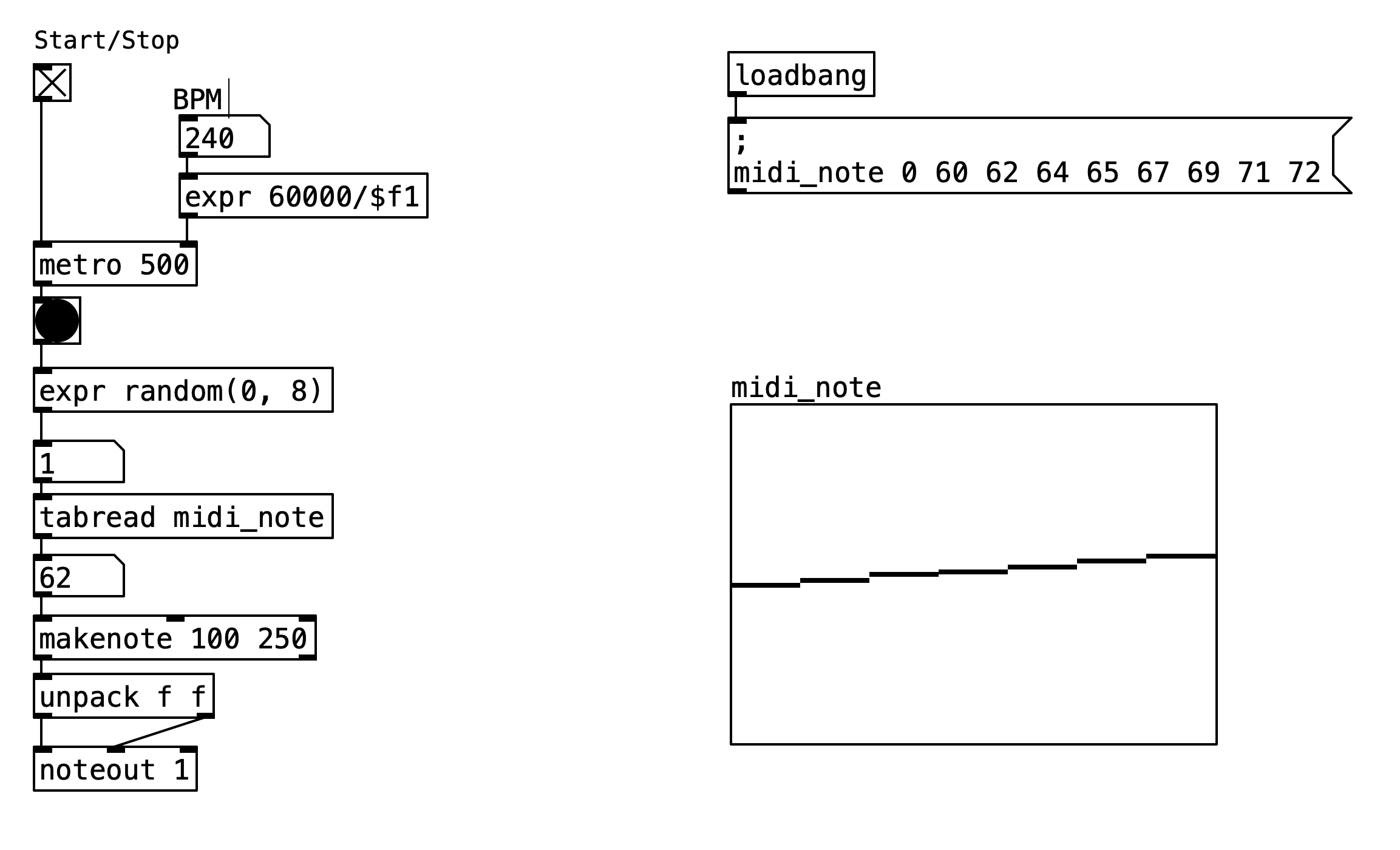
Fig. Random step sequencer patch showing the integration of random number generation with array-based note storage and MIDI output, creating unpredictable yet musically coherent patterns from predefined harmonic material.

The random step sequencer represents an evolution of the basic sequential approach to rhythm generation. Instead of following a predictable linear progression through stored note values, this implementation introduces stochastic elements that create unpredictable yet musically coherent patterns. This patch demonstrates how randomization can be integrated into sequencing systems to generate non-repetitive musical content while maintaining the fundamental structure of step-based sequencing.

2.3.1 Patch Overview

The random step sequencer patch builds upon the foundational concepts of the basic 8-step sequencer while introducing a crucial modification: the step advancement mechanism is replaced with a random selection process. Rather than incrementing through array indices sequentially, the system generates random index values that point to different positions within the stored note sequence. This approach maintains the same timing control, array-based storage, and MIDI output capabilities as the sequential version, but produces entirely different musical results due to the non-linear access pattern.

The architecture preserves the linear signal flow from user controls to MIDI output, but introduces a random number generator at the critical junction where step advancement occurs. The timing engine continues to use Pd’s metro object as the primary clock source, but each timing pulse now triggers a random selection rather than a predictable increment. This modification transforms the sequencer from a deterministic system into a probabilistic one, where the same stored sequence can produce infinite variations in playback order.

The interface maintains the same visual feedback mechanisms as the sequential version, displaying both the randomly selected step index and the corresponding MIDI note value. The tempo control system remains unchanged, allowing users to adjust playback speed while experiencing the unpredictable note selection patterns that emerge from the randomization process.

2.3.2 Data Flow

flowchart TD
    A[Start/Stop Toggle] --> B[Metro Object]
    C[BPM Slider] --> D[BPM to ms Conversion]
    D --> B
    B --> E[Random Generator]
    E --> F[Random Index 0-7]
    F --> G[Step Index Display]
    G --> H[Array Lookup]
    H --> I[MIDI Note Display]
    I --> J[Makenote Object]
    J --> K[MIDI Output]
    L[Loadbang] --> M[Array Initialization]
    M --> H

The operational sequence begins identically to the sequential version, with the user activating the start/stop toggle to enable metro object timing generation. The BPM slider continues to control tempo through the same mathematical conversion formula 60000/$f1, ensuring consistent timing accuracy regardless of the randomization occurring downstream.

The fundamental difference emerges at the step generation stage. Instead of using a counter that increments predictably, each timing pulse from the metro object triggers a random number generator implemented with the expr random(0, 8) object. This expression generates random integers between 0 and 7 (inclusive), providing equal probability access to any position within the 8-element note array. The random selection occurs independently for each timing pulse, meaning the same index can be selected multiple times in succession, or the system might skip certain indices entirely during any given playback session.

The randomly generated index serves the same dual purpose as in the sequential version: providing immediate visual feedback through a numeric display and functioning as the lookup key for array access. The tabread midi_note object retrieves the MIDI note value corresponding to the randomly selected index, creating an unpredictable sequence of pitches from the stored scale pattern.

The subsequent processing stages remain unchanged from the sequential implementation. The retrieved MIDI note value is displayed numerically, then processed through the makenote object with the same fixed velocity (100) and duration (250 milliseconds) parameters. The resulting MIDI messages are transmitted through the noteout object to MIDI channel 1, maintaining full compatibility with external synthesizers and recording systems.

The array initialization process follows the identical pattern established in the sequential version, using a loadbang object to populate the midi_note array with the C major scale sequence 60 62 64 65 67 69 71 72 at patch startup. This ensures immediate availability of musical content regardless of the randomization method employed.

2.3.3 Key Objects and Their Roles

The following table summarizes the essential objects used in the random step sequencer implementation, highlighting the specific changes from the sequential version:

Object	Purpose
`metro`	Timing engine that generates regular pulses
`expr 60000/$f1`	Converts BPM to milliseconds for metro timing
`expr random(0, 8)`	Generates random indices from 0 to 7
`tabread midi_note`	Reads MIDI note values from the array
`makenote`	Creates MIDI note-on/off messages with velocity and duration
`unpack f f`	Separates MIDI note and velocity values
`noteout`	Transmits MIDI messages to specified channel
`array midi_note`	Stores the sequence of MIDI note values

This implementation demonstrates how simple modifications to algorithmic components can produce dramatically different results. The random step sequencer maintains all the practical advantages of the sequential version—including real-time tempo control, visual feedback, and MIDI compatibility—while introducing the creative possibilities inherent in stochastic processes. The resulting system serves as an excellent foundation for exploring probability-based composition techniques and can be extended with weighted random selection, controlled randomness, or hybrid deterministic-stochastic approaches.

2.4 Piano Phase (Steve Reich)

View Piano Phase Score (S. Reich)

Design patterns are abstractions that capture idiomatic tendencies of practices and processes. These abstractions are embedded in live coding languages as functions and syntax, allowing for the reuse of these practices in new projects (Brown 2023).

Piano Phase is an example of “music as a gradual process,” as Reich stated in his essay from 1968.(Reich 2002). In it, Reich described his interest in using processes to generate music, particularly noting how the process is perceived by the listener. Processes are deterministic: a description of the process can describe an entire whole composition. In other words, once the basic pattern and the phase process have been defined, the music consists itself. Reich called the unexpected ways change occurred via the process “by-products”, formed by the superimposition of patterns. The superimpositions form sub-melodies, often spontaneously due to echo, resonance, dynamics, and tempo, and the general perception of the listener(Epstein 1986). Piano Phase led to several breakthroughs that would mark Reich’s future compositions. The first is the discovery of using simple but flexible harmonic material, which produces remarkable musical results when phasing occurs. The use of 12-note or 12-division patterns in Piano Phase proved to be successful, and Reich would re-use it in Clapping Music and Music for 18 Musicians. Another novelty is the appearance of rhythmic ambiguity during phasing of a basic pattern. The rhythmic perception during phasing can vary considerably, from being very simple (in-phase), to complex and intricate.

The first section of Piano Phase has been the section studied most by musicologists. A property of the first section of phase cycle is that it is symmetric, which results in identical patterns half-way through the phase cycle (Epstein 1986). Piano Phase can be conceived as an algorithm. Starting with two pianos playing the same sequence of notes at the same speed, one of the pianists begins to gradually accelerate their tempo.

When the separation between the notes played by both pianos reaches a fraction of a note’s duration, the phase is shifted and the cycle repeats. This process continues endlessly, creating a hypnotic effect of rhythmic phasing that evolves over time as an infinite sequence of iterations.

2.4.1 Algorithm Formulation (pseudo code)

1. Initialize two pianists with the same note sequence.
2. Set an initial tempo for both pianists.
3. Repeat until the desired phase is reached:
     a. Gradually increase the second pianist's tempo.
     b. Compare note positions between both pianists.
     c. When the separation between the notes reaches a fraction of a note’s duration, invert the phase.
     d. Continue playback.
4. Repeat the cycle indefinitely to create a continuous and evolving rhythmic phasing effect.

2.4.2 Piano Phase Implementation in Pd

Fig. Piano Phase patch demonstrating phasing process through two sequencers with different metro intervals, visualized with hradio step indicators and MIDI output for each voice. — Fig. *Piano Phase* patch demonstrating phasing process through two sequencers with different metro intervals, visualized with hradio step indicators and MIDI output for each voice.

2.4.3 Patch Overview

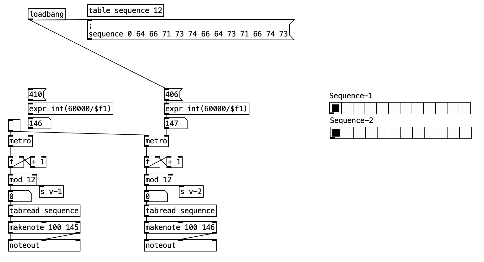
The piano-phase.pd patch implements a minimalist phasing process inspired by Steve Reich’s Piano Phase. It uses two parallel sequencers, each reading from the same melodic sequence but advancing at slightly different rates. This gradual tempo difference causes the two sequences to drift out of phase, creating evolving rhythmic and melodic patterns.

2.4.3.1 Sequence Data

[table sequence 12]

The sequence is stored in a table named sequence with 12 MIDI note values:

64 66 71 73 74 66 64 73 71 66 74 73

This pattern is initialized at patch load.

2.4.4 Data Flow

flowchart TD
    Start([Start/Stop]) --> M1[Clock 1 410ms]
    Start --> M2[Clock 2 406ms]
    M1 --> C1[Counter 1]
    M2 --> C2[Counter 2]
    C1 --> T1[read sequence]
    C2 --> T2[read sequence]
    T1 --> MK1[MIDI noteout]
    T2 --> MK2[MIDI noteout]

The operation of the Piano Phase patch begins with an initialization stage, triggered by a loadbang object when the patch is opened. This setup phase populates the shared sequence table with its 12 predefined MIDI note values. Simultaneously, the two metro objects, which serve as the independent clocks for each of the two parallel “pianists” or sequencers, are configured with their distinct time intervals: the left sequencer’s metro is set to 410 milliseconds, and the right sequencer’s metro to a slightly faster 406 milliseconds. A single toggle control allows the user to start or stop both metro objects concurrently, initiating or halting the phasing process.

Once activated, each metro object begins to output a stream of bangs at its specified interval. These bangs drive separate but structurally identical sequencing logics. For each sequencer, its respective metro pulse triggers a counter. This counter, typically implemented with a combination of f (float atom), + 1 (increment), and mod 12 (modulo) objects, advances its step index from 0 to 11. Upon reaching 11, the modulo operation ensures it wraps back to 0, allowing the 12-step sequence to loop continuously.

The current step index generated by each counter is then used to read a MIDI note value from the shared sequence table via a tabread sequence object. Thus, each sequencer independently fetches notes from the same melodic pattern according to its own current position. The retrieved MIDI note from each sequencer is subsequently processed by its own makenote object, which formats it into standard MIDI note-on and note-off messages, typically with a predefined velocity and duration. These MIDI messages are then sent to separate noteout objects, allowing the two voices to be routed to different MIDI channels or instruments if desired, or simply to play concurrently. Visual feedback for each sequencer’s current step is provided by a dedicated hradio object, which updates in sync with its counter.

The core phasing effect emerges from the slight discrepancy in the metro intervals. Because the right sequencer’s clock (406 ms) is marginally faster than the left’s (410 ms), its counter advances more rapidly. This causes the right sequencer’s melodic line to gradually “pull ahead” of the left. Over time, this desynchronization means the two identical melodic patterns are heard starting at different points relative to each other, creating complex, shifting rhythmic and harmonic interactions. This process continues cyclically: the faster sequence eventually “laps” the slower one, bringing them back into unison before they begin to drift apart again, perpetuating the mesmerizing phasing phenomenon central to Reich’s composition.

Phasing Effect

The right sequencer is slightly faster, so its step index gradually shifts ahead of the left sequencer.
Over time, the two sequences drift out of phase, producing new rhythmic and melodic combinations.
Eventually, the faster sequencer laps the slower one, and the process repeats.

2.4.5 Key Objects and Their Roles

Object	Purpose
metro	Sets the timing for each sequencer
expr int(60000/$f1)	Converts BPM to milliseconds
f, + 1, mod 12	Advances and wraps the step index
tabread sequence	Reads the current note from the sequence
makenote	Generates MIDI note-on/off with duration
noteout	Sends MIDI notes to the output device

2.5 Random Melody Generator

The patch demonstrates how to generate a melody using a musical scale, store it in an array, and play it back using MIDI.

Fig. Random melody generator patch showing scale definition, algorithmic note selection, array storage, and MIDI playback system for creating melodic sequences from predefined harmonic material.

2.5.1 Patch Overview

The Random Melody Generator patch demonstrates a comprehensive approach to algorithmic composition. This implementation showcases how to generate melodic content using musical scales, store the generated material in arrays for manipulation, and create a playback system with MIDI output capabilities.

The patch architecture is built around several interconnected functional blocks that work together to create a complete generative music system. The first component handles scale definition and melody generation, where musical scales are defined as interval patterns and used as the foundation for creating new melodic material. The melody storage system utilizes array objects to hold the generated sequences, providing both data persistence and visual feedback. The playback control mechanism employs metronome objects and indexing systems to sequence through the stored melodies at controllable tempos. Finally, the MIDI output section transforms the stored note data into playable MIDI messages that can be sent to external synthesizers or software instruments.

This modular design approach allows for easy modification and extension of the system. Each functional block can be adjusted independently, enabling composers and sound designers to experiment with different scales, generation algorithms, storage methods, and playback configurations without affecting the overall system stability.

2.5.2 Data Flow

flowchart TD
    S[Scale Message] --> L[list Append]
    L --> R[random + Offset]
    R --> M[Modulo/Indexing]
    M --> A[Melody Array]
    A --> P[Playback - metro, tabread]
    P --> MN[makenote]
    MN --> NO[noteout]

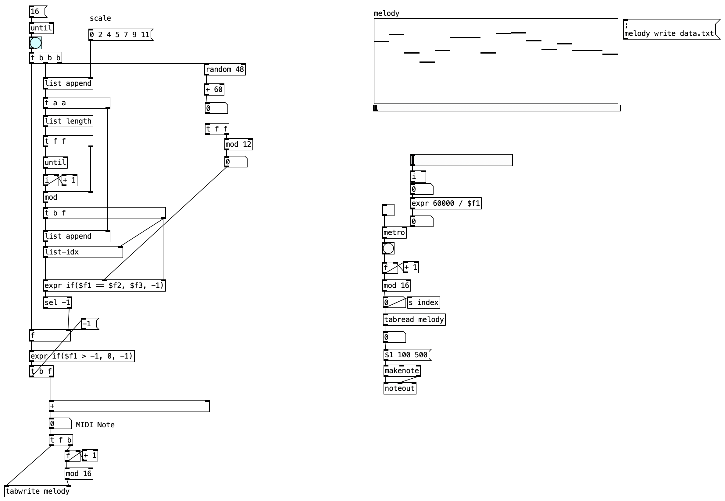
The scale definition process begins with a message box containing the fundamental building blocks of Western harmony represented as semitone intervals. The example scale 0 2 4 5 7 9 11 represents a major scale pattern, where each number corresponds to a specific semitone distance from a root note. This intervallic approach provides flexibility, as the same pattern can be transposed to any key by simply changing the root note offset. The scale intervals are processed through list manipulation objects, which append the values to an internal list structure and calculate the scale’s length for use in subsequent random selection processes.

The following table illustrates the mapping of musical notes to their corresponding intervals in semitones, which is crucial for understanding how the scale is constructed and how notes are generated from it.

Note	Interval
C	`0`
C# / Db	`1`
D	`2`
D# / Eb	`3`
E	`4`
F	`5`
F# / Gb	`6`
G	`7`
G# / Ab	`8`
A	`9`
A# / Bb	`10`
B	`11`

The random note selection mechanism forms the core of the melodic generation process. A random number generator produces values between 0 and 47, which are then shifted upward by 60 to place the resulting MIDI notes in a musically appropriate range around middle C. This range selection ensures that generated melodies will fall within a playable range for most instruments and remain audible in typical monitoring setups. The random values are then mapped to the predefined scale using modulo operations and list indexing, ensuring that all generated notes conform to the harmonic framework established by the scale definition.

The melody construction process utilizes looping mechanisms, specifically the until, i, and + 1 objects, to generate sequences of predetermined length. Each iteration of the loop calculates a new note based on the scale mapping process and stores the result in a growing list structure. This approach allows for the creation of melodic phrases of any desired length, from short motifs to extended melodic lines. The deterministic nature of the loop structure ensures predictable behavior while the random element within each iteration provides the variability necessary for interesting melodic content.

For melody storage, the patch employs array system, specifically an array named melody that serves as both a data repository and a visual display element. The generated melodic sequences are written to this array using the tabwrite object, which provides indexed storage capabilities. The array’s visual representation appears as a graph within the patch interface, allowing users to see the melodic contour and note relationships in real-time. This visual feedback proves invaluable for understanding the characteristics of generated material and making informed decisions about parameter adjustments.

The playback control system centers around a metro object that functions as a digital metronome, generating regular timing pulses that drive the sequencing process. The tempo of these pulses is controlled by a horizontal slider interface element, providing real-time tempo adjustment capabilities. Each pulse from the metronome advances an index counter that points to the next position in the melody array. This indexing system automatically wraps around to the beginning when it reaches the end of the stored sequence, creating seamless looping playback that continues indefinitely until stopped by the user.

The MIDI output stage transforms the stored melodic data into standard MIDI protocol messages that can interface with external hardware and software. The note values retrieved from the array are processed through a makenote object, which creates properly formatted MIDI note-on and note-off messages with specified velocity and duration parameters. These parameters can be adjusted to affect the musical expression of the playback, with velocity controlling the apparent loudness or intensity of notes and duration determining their length. The final noteout object handles the actual transmission of MIDI data to the system’s MIDI routing infrastructure, where it can be directed to synthesizers, samplers, or recording software.

2.5.3 Key Objects and Their Roles

Object	Purpose
`random 48`	Generates random note indices
`+ 60`	Shifts notes to a higher MIDI octave
`mod 12`	Maps notes to scale degrees
`list-idx`	Retrieves scale degree from the list
`tabwrite`	Writes notes to the `melody` array
`metro`	Controls playback timing
`tabread`	Reads notes from the `melody` array
`makenote`	Creates MIDI notes with velocity/duration
`noteout`	Sends MIDI notes to output

The integration of these components creates a flexible and powerful tool for algorithmic composition. The system can generate new melodic material on demand, store multiple variations for comparison, and play back the results in real-time with full MIDI compatibility. This makes it suitable for both experimental composition work and practical music production applications, where generated material can serve as inspiration, accompaniment, or the foundation for further development.

2.6 The Euclidean Algorithm Generates Traditional Musical Rhythms

See original paper

The Euclidean rhythm in music was discovered by Godfried Toussaint in 2004 and is described in a 2005 paper “The Euclidean Algorithm Generates Traditional Musical Rhythms” (Toussaint 2005). The paper presents a method for generating rhythms that are evenly distributed over a given time span, using the Euclidean algorithm. This method is particularly relevant in the context of world music, where such rhythms are often found. The Euclidean algorithm (as presented in Euclid’s Elements) calculates the greatest common divisor of two given integers. It is shown here that the structure of the Euclidean algorithm can be used to efficiently generate a wide variety of rhythms used as timelines (ostinatos) in sub-Saharan African music in particular, and world music in general. These rhythms, here called Euclidean rhythms, have the property that their onset patterns are distributed as evenly as possible. Euclidean rhythms also find application in nuclear physics accelerators and computer science and are closely related to several families of words and sequences of interest in the combinatorics of words, such as Euclidean strings, with which the rhythms are compared (Toussaint 2005).

2.6.1 Hypothesis

Several researchers have observed that rhythms in traditional world music tend to exhibit patterns distributed as regularly or evenly as possible. The hypothesis is that the Euclidean algorithm can be used to generate these rhythms. According to the hypothesis, the Euclidean algorithm can be used to generate rhythms that are evenly distributed over a given time span. This is particularly relevant in the context of world music, where such rhythms are often found. The following is a summary of the main points:

Patterns of maximal evenness can be described using the Euclidean algorithm on the greatest common divisor of two integers.

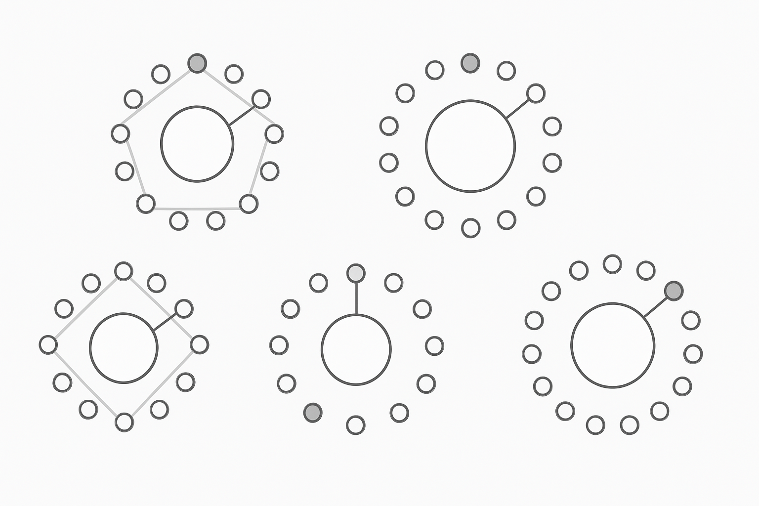
2.6.2 Patterns of Maximal Evenness

The Pattern of Maximal Evenness is a concept used in music theory to create Euclidean rhythms. Euclidean rhythms are rhythmic patterns that evenly distribute beats over a time cycle.

In essence, the Pattern of Maximal Evenness seeks to distribute a specific number of beats evenly within a given time span. This is achieved by dividing the time into equal parts and assigning beats to these divisions uniformly.

Example:

x = beat

· = rest

[×· ×· ×· ×· ] → [1 0 1 0 1 0 1 0]

(8,4) = 4 beats evenly distributed over 8 pulses

[×· ·×· ·×·] → [1 0 0 1 0 0 1 0]

(8,3) = 3 beats evenly distributed over 8 pulses

2.6.3 Euclidean Algorithm

One of the oldest known algorithms, described in Euclid’s Elements (around 300 BCE) in Proposition 2 of Book VII, now known as the Euclidean algorithm, calculates the greatest common divisor of two given integers.

The idea is very simple. The smaller number is repeatedly subtracted from the larger until the larger becomes zero or smaller than the smaller one, in which case it becomes the remainder. This remainder is then repeatedly subtracted from the smaller number to obtain a new remainder. This process continues until the remainder is zero.

To be more precise, consider the numbers 5 and 8 as an example:

Step	Operation	Equation	Quotient	Remainder
1	Divide 8 by 5	\[8 = 1 \cdot 5 + 3\]	1	3
2	Divide 5 by 3	\[5 = 1 \cdot 3 + 2\]	1	2
3	Divide 3 by 2	\[3 = 1 \cdot 2 + 1\]	1	1
4	Divide 2 by 1	\[2 = 2 \cdot 1 + 0\]	2	0

The idea is to keep dividing the previous divisor by the remainder obtained in each step until the remainder is 0. When we reach a remainder of 0, the previous divisor is the greatest common divisor of the two numbers.

In short, the process can be seen as a sequence of equations:

\[\begin{align*} 8 &= (1)\cdot(5) + 3 \\ 5 &= (1)\cdot(3) + 2 \\ 3 &= (1)\cdot(2) + 1 \\ 2 &= (1)\cdot(2) + 0 \end{align*}\]

Note: 8 = (1) . (5) + 3 means that 8 is divided by 5 once, yielding a quotient of 1 and a remainder of 3.

In essence, it involves successive divisions to find the greatest common divisor of two positive numbers (GCD from now on).

The GCD of two numbers a and b, assuming a > b, is found by first dividing a by b, and obtaining the remainder r.

The GCD of a and b is the same as that of b and r. When we divide a by b, we obtain a quotient c and a remainder r such that:

$a = c \cdot b + r$

Examples:

Let’s compute the GCD of 17 and 7.

Since 17 = 7 · 2 + 3, then GCD(17, 7) is equal to GCD(7, 3). Again, since 7 = 3 · 2 + 1, then GCD(7, 3) is equal to GCD(3, 1). Here, it is clear that the GCD between 3 and 1 is simply 1. Therefore, the GCD between 17 and 7 is also 1.

\[\text{GCD}(17,7) = 1\] \[17 = 7 \cdot 2 + 3\] \[7 = 3 \cdot 2 + 1\] \[3 = 1 \cdot 3 + 0\]

Another example:

\[\text{GCD}(8,3) = 1\] \[8 = 3 \cdot 2 + 2\] \[3 = 2 \cdot 1 + 1\] \[2 = 1 \cdot 2 + 0\]

2.6.4 How does computing the GCD turn into maximally even distributed patterns?

Represent a binary sequence of k ones [1] and n − k zeros [0], where each [0] bit represents a time interval and the ones [1] indicate signal triggers.

The problem then reduces to:

Construct a binary sequence of n bits with k ones such that the ones are distributed as evenly as possible among the zeros.

A simple case is when k evenly divides n (with no remainder), in which case we should place ones every n/k bits. For example, if n = 16 and k = 4, then the solution is:

\[[1 0 0 0 1 0 0 0 1 0 0 0 1 0 0 0]\]

This case corresponds to n and k having a common divisor of k (in this case 4).

More generally, if the greatest common divisor between n and k is g, we would expect the solution to decompose into g repetitions of a sequence of n/g bits. This connection with greatest common divisors suggests that we could compute a maximally even rhythm using an algorithm like Euclid’s.

2.6.4.1 Example (13, 5)

Let’s consider a sequence with n = 13 and k = 5.

Since 13 − 5 = 8, we start with a sequence consisting of 5 ones, followed by 8 zeros, which can be thought of as 13 one-bit sequences:

\[[1 1 1 1 1 0 0 0 0 0 0 0 0]\]

We begin moving zeros by placing one zero after each one, creating five 2-bit sequences, with three remaining zeros:

\[[10] [10] [10] [10] [10] [0] [0] [0]\]

\[13 = 5 · 2 + 3\]

Then we distribute the three remaining zeros similarly, placing a [0] after each [10] sequence:

\[[100] [100] [100] [10] [10]\]

\[5 = 3 · 1 + 2\]

We now have three 3-bit sequences, and a remainder of two 2-bit sequences. So we continue the same way, placing one [10] after each [100]:

\[[10010] [10010] [100]\]

\[3 = 2 · 1 + 1\]

The process stops when the remainder consists of a single sequence (here, [100]), or we run out of zeros.

The final sequence is, therefore, the concatenation of [10010], [10010], and [100]:

\[[1 0 0 1 0 1 0 0 1 0 1 0 0]\]

\[2 = 1 · 2 + 0\]

2.6.4.2 Example (17, 7)

Suppose we have 17 pulses and want to evenly distribute 7 beats over them.

1. We align the number of beats and silences (7 ones and 10 zeros):

\[[1 1 1 1 1 1 1 0 0 0 0 0 0 0 0 0 0]\]

\[[1 1 1 1 1 1 1] [0 0 0 0 0 0 0 0 0 0]\]

2. We form 7 groups, corresponding to the division of 17 by 7; we get 7 groups of [1 0] and 3 remaining zeros [000], which means the next step forms 3 groups until only one or zero groups remain.

\[ [1 0] [1 0] [1 0] [1 0] [1 0] [1 0] [1 0] [0] [0] [0]\]

\[ 17 = 7 \cdot 2 + 3\]

1	1	1	1	1	1	1	0 0 0
0	0	0	0	0	0	0

3. Again, this corresponds to dividing 7 by 3. In our case, we are left with only one group and we are done.

\[ [1 0 0] [1 0 0] [1 0 0] [1 0] [1 0] [1 0] [1 0]\]

1	1	1	1	1	1	1
0	0	0	0	0	0	0
0	0	0

\[ [1 0 0 1 0] [1 0 1 0 0] [1 0 0 1 0] [1 0]\]

\[ 7 = 3 · 2 + 1\]

1	1	1	1
0	0	0	0	0	0	0
0	0	0
1	1	1
0	0	0

4. Finally, the rhythm is obtained by reading the grouping column by column, from left to right, step by step.

\[ [1 0 0 1 0 1 0 0 1 0 1 0 0 1 0 1 0]\]

\[ 3 = 1 · 3 + 0\]

2.6.5 Implementation in Pd - Euclidean sequencer

The following code implements the Euclidean algorithm in Pd to generate a Euclidean rhythm. The algorithm is based on the mathematical formula:

\[(\text{index} \cdot \text{hits}) \% \text{ steps} < \text{notes}\]

where:

$\text{index}$ = index of the Euclidean series (array)
$\text{hits}$ = number of notes to be played
$\text{steps}$ = array size
$\text{notes}$ = threshold for comparison

Yoy can check this Euclidean rhythm demo in order to interact and see how the algorithm works.

2.6.5.1 Understanding the Mathematical Formula

The formula (index * hits) % steps < hits provides a simple and efficient way to approximate the distribution of pulses (or beats) over a sequence of discrete steps. It works by multiplying the current position (represented by index) by the total number of hits (pulses) desired. This result is then taken modulo the total number of steps to ensure it wraps around properly in a cyclical pattern. Finally, the result of this modulo operation is compared to the number of hits. If the condition is true, we place a beat at that position; otherwise, we place a rest.

This method produces a rhythm by relying on modular arithmetic. The result is a mathematically regular distribution of beats that often approximates what we expect from an even rhythmic distribution. However, it does so without any recursive logic or iteration—it simply applies a consistent rule to each step in isolation. This makes the formula extremely efficient: it runs in constant time for any position, and it does not require any memory to store the pattern.

2.6.5.2 The Bjorklund Algorithm Explained

In contrast, the Bjorklund algorithm is a more sophisticated procedure rooted in the Euclidean algorithm for computing the greatest common divisor (GCD). This algorithm begins with two values: the number of pulses (beats) and the number of rests (steps minus beats). It then recursively groups these elements in a way that maximizes the evenness of their distribution.

The method proceeds by repeatedly pairing elements—first grouping pulses with rests, then regrouping the leftovers, and so on—until the sequence cannot be subdivided further. The final pattern emerges from this recursive grouping, and it is typically rotated so that it starts with a pulse. The result is a rhythm that is maximally even, meaning that the beats are spaced as equally as possible given the constraints.

This process, while more computationally demanding and conceptually complex, produces the canonical Euclidean rhythms often cited in academic and musical literature.

2.6.5.3 Comparing the Formula and the Algorithm

The core difference between the two approaches lies in how they arrive at the rhythmic pattern. The mathematical formula provides a direct, position-based method for determining beat placement. It does not take into account the context of previous or future beats—it treats each step in isolation. This is why it is so fast and well-suited for real-time applications, such as live audio processing in Pd or other creative coding environments.

The Bjorklund algorithm, on the other hand, is concerned with the global structure of the pattern. It ensures that beats are distributed with maximal evenness and follows a well-defined sequence of operations that are both recursive and stateful. This means it needs to store and manipulate arrays of data to arrive at the final rhythm. The computational complexity of this algorithm is higher, and it is not as straightforward to implement, but the results are musically and mathematically robust.

One major distinction is that the formula often produces a rotated version of the Bjorklund rhythm. That is, while the number and spacing of beats may be similar, the starting position may differ. The Bjorklund rhythm always starts with a pulse, ensuring that it adheres to a particular musical convention, while the formula does not guarantee this.

Another important distinction lies in the distribution logic. The formula uses a fixed mathematical rule to space out the beats, leading to regular but not necessarily optimal placement. The Bjorklund algorithm, however, iteratively rearranges beats and rests to achieve the best possible balance.

2.6.5.4 A Concrete Example: (13, 5)

Let’s consider the case of 13 steps with 5 beats.

Using the mathematical formula, we apply (index * 5) % 13 < 5 for each position:

Pattern: 1 0 0 1 0 0 1 0 1 0 0 1 0

In contrast, the Bjorklund algorithm produces:

Pattern: 1 0 1 0 0 1 0 1 0 0 1 0 0

Both patterns contain five beats. Both distribute them fairly evenly. But the Bjorklund version achieves a more perceptually even spacing and aligns with theoretical expectations. The formula result is essentially a rotated variant.

In summary, the formula (index * hits) % steps < hits offers a pragmatic and computationally efficient way to generate rhythm patterns that resemble Euclidean rhythms. It is well-suited for real-time use cases and environments where simplicity and speed are more important than strict accuracy. In contrast, the Bjorklund algorithm provides a mathematically rigorous method for generating rhythms with maximal evenness. It aligns with canonical definitions and is favored in theoretical and compositional contexts.The choice between these methods depends on your priorities: use the formula for lightweight, real-time approximation, and use Bjorklund when you need precision and adherence to the canonical Euclidean model.

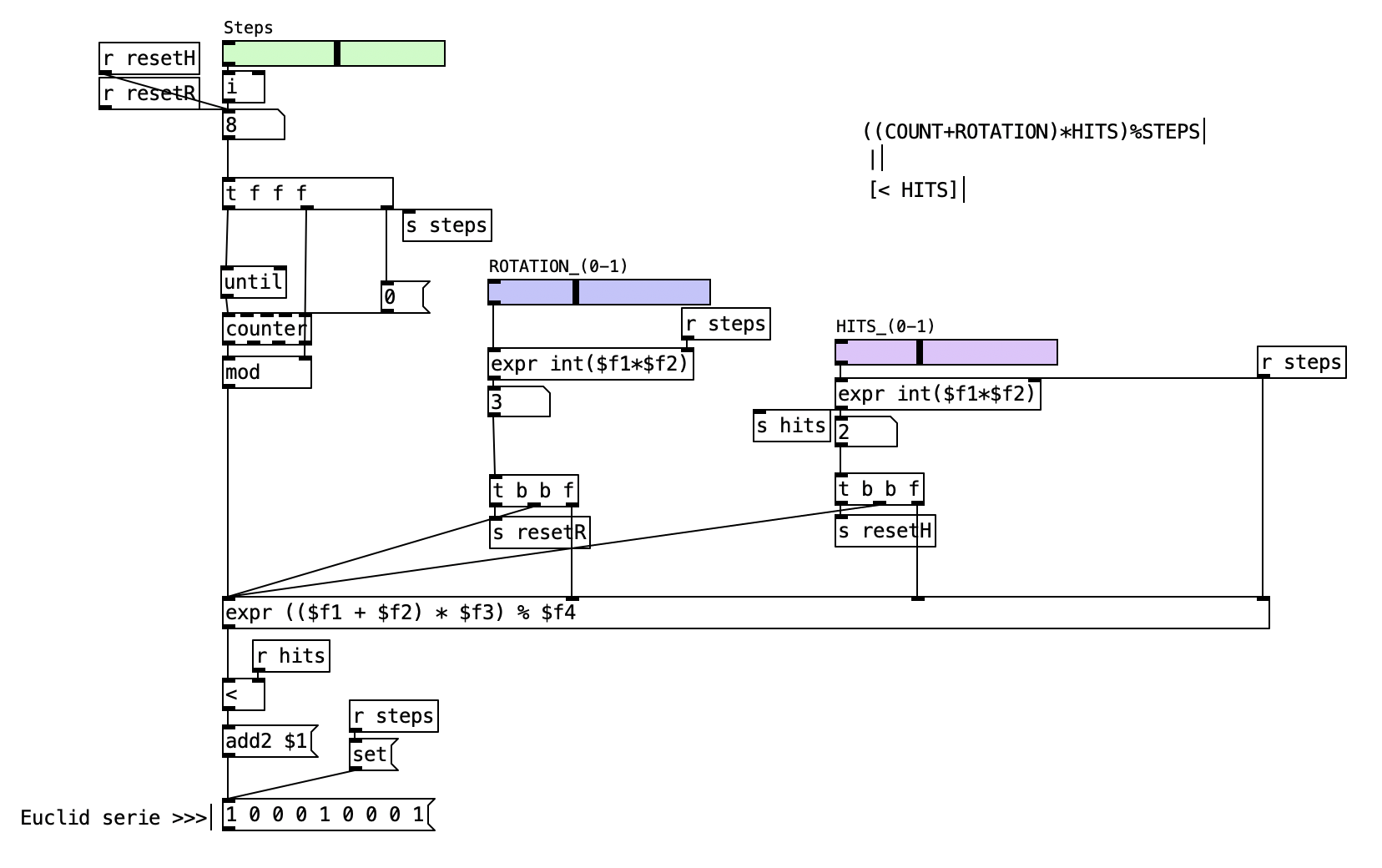
2.6.6 Euclidean Rhythm Generator

This section provides a detailed explanation of the Euclidean-basic-Serie.pd patch. This Pd patch demonstrates how to generate Euclidean rhythms using a straightforward mathematical formula.

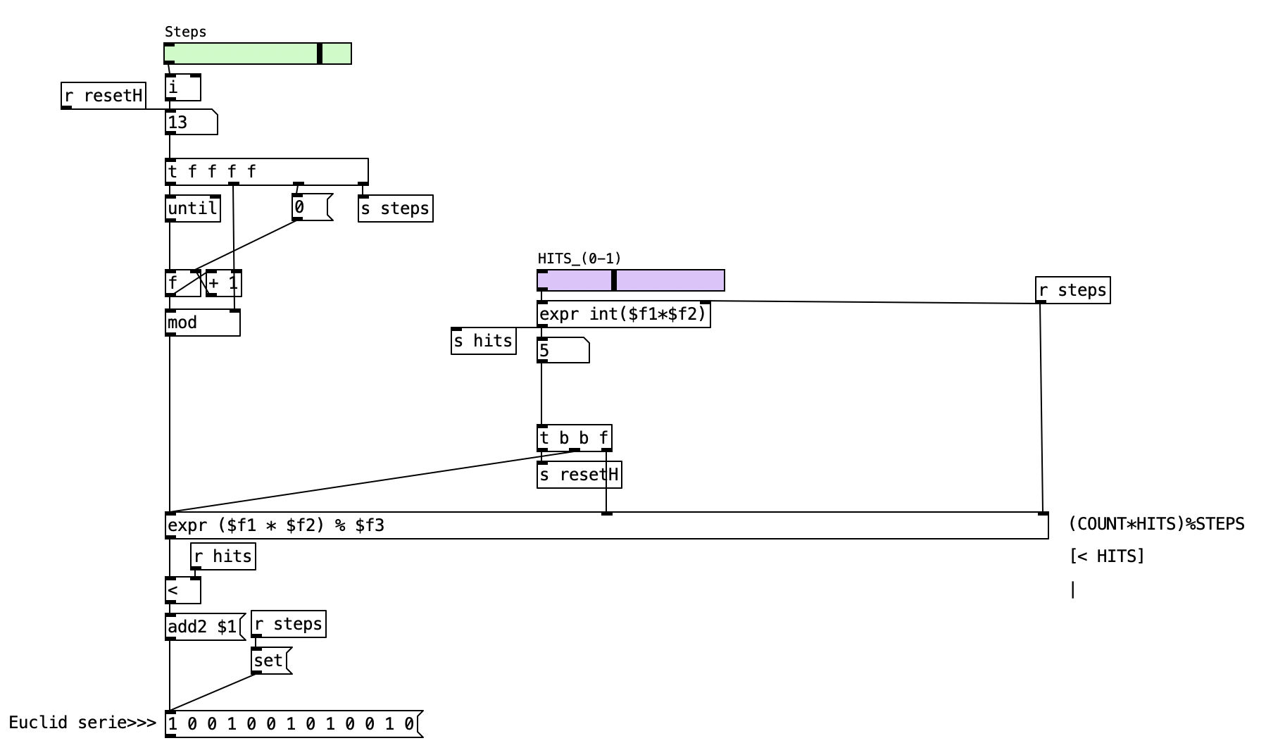
Euclidean rhythm generator patch showing step and hit parameter controls, mathematical formula calculation, and pattern output display for generating evenly distributed rhythmic sequences.

2.6.6.1 Patch Overview

The patch is structured into several functional blocks. First, there are controls for setting the number of steps and the number of hits (pulses). Next, the patch calculates the Euclidean pattern using a mathematical formula.

(index * hits ) % steps
↓
[< notes]

Finally, the resulting pattern is output and visualized as a list of pulses and rests.

2.6.6.2 Data Flow

flowchart TD
    S[Steps Slider] --> A[Step Counter]
    H[Hits Slider] --> B[Hits Value]
    A --> C[Euclidean Formula: index * hits % steps]
    B --> C
    C --> D[Compare < hits]
    D --> E[Pattern List]
    E --> F[Output/Display]

The process begins with the user setting the number of steps in the sequence using a horizontal slider labeled “Steps.” This determines the total length of the rhythmic cycle. The user also sets the number of hits, or pulses, using another slider labeled “HITS.” These two values are stored and sent to the rest of the patch, where they are used to calculate the rhythmic pattern.

Once the parameters are set, the patch uses a loop, implemented with the until object, to iterate through each step index from 0 up to one less than the total number of steps. For each index, the patch calculates a value using the formula (index * hits) % steps. This formula determines the position of each pulse within the cycle by multiplying the current index by the number of hits and taking the result modulo the total number of steps. The result of this calculation is then compared to the number of hits. If the result is less than the number of hits, a pulse (represented by a 1) is added to the pattern. Otherwise, a rest (represented by a 0) is added. This process is repeated for every step in the sequence, gradually building up the complete Euclidean rhythm as a list of ones and zeros.

After the pattern has been calculated, it is displayed as a list, allowing you to see the sequence of pulses and rests. The patch also includes a reset mechanism, so that the pattern can be recalculated and updated whenever the user changes the number of steps or hits.

2.6.6.3 Example: (Steps = 13, Hits = 5)

To illustrate how the patch works, consider the case where the number of steps is 13 and the number of hits is 5. The following table shows the calculation for each step:

Index	Calculation	Result	< Hits?	Output
0	(0 * 5) % 13 = 0	0	Yes	1
1	(1 * 5) % 13 = 5	5	Yes	1
2	(2 * 5) % 13 = 10	10	No	0
3	(3 * 5) % 13 = 2	2	Yes	1
4	(4 * 5) % 13 = 7	7	No	0
5	(5 * 5) % 13 = 12	12	No	0
6	(6 * 5) % 13 = 4	4	Yes	1
7	(7 * 5) % 13 = 9	9	No	0
8	(8 * 5) % 13 = 1	1	Yes	1
9	(9 * 5) % 13 = 6	6	No	0
10	(10 * 5) % 13 = 11	11	No	0
11	(11 * 5) % 13 = 3	3	Yes	1
12	(12 * 5) % 13 = 8	8	No	0

The resulting pattern is:
\[1 1 0 1 0 0 1 0 1 0 0 1 0\]

This sequence distributes five pulses as evenly as possible across thirteen steps.

2.6.6.4 Key Objects and Their Roles

The following table summarizes the key objects used in the patch and their roles:

Object	Purpose
`until`	Loops through each step index
`expr`	Calculates `(index * hits) % steps`
`<`	Compares result to hits, outputs 1 or 0
`add2`	Appends each result to the output pattern list
`mod`	Ensures index wraps around for correct calculation

2.6.7 Euclidean Rotation Generator

This section explains the Euclidean-Rotation.pd patch. This Pd patch builds on the basic Euclidean rhythm generator by introducing a rotation parameter, allowing you to shift the starting point of the rhythm pattern. This feature is useful for exploring different phase relationships and rhythmic variations without changing the underlying distribution of pulses.

Fig. Euclidean rotation generator patch showing enhanced rhythm control with rotation parameter for cyclical pattern shifting and phase exploration.

2.6.7.1 Patch Overview

The patch allows you to set the number of steps, the number of hits (pulses), and the rotation amount. The rotation parameter shifts the pattern cyclically, so the rhythm can start at any point in the sequence. The patch calculates the Euclidean pattern using a formula that incorporates the rotation, and then outputs the resulting pattern for visualization and further use.

The following diagram illustrates the data flow for the rhythm and rotation:

flowchart TD
    Steps[Steps Slider] --> Counter[Step Counter]
    Hits[Hits Slider] --> HitsVal[Hits Value]
    Rot[Rotation Slider] --> RotVal[Rotation Value]
    Counter --> Formula[Euclidean Formula: index_plus_rotation_times_hits_mod_steps]
    RotVal --> Formula
    HitsVal --> Formula
    Formula --> Compare[Compare to Hits]
    Compare --> Pattern[Pattern List]
    Pattern --> Output[Output/Display]

2.6.7.2 Data Flow

The process begins with the user setting the number of steps, hits, and rotation using horizontal sliders. The steps slider determines the total length of the rhythmic cycle, the hits slider sets the number of pulses to be distributed, and the rotation slider specifies how many positions to shift the pattern.

A loop, implemented with the until object and a counter, iterates through each step index. For each index, the patch calculates the value using the formula ((index + rotation) * hits) % steps. This formula determines the position of each pulse within the cycle, taking into account the rotation. The result is then compared to the number of hits: if it is less than the number of hits, a pulse (represented by a 1) is added to the pattern; otherwise, a rest (represented by a 0) is added. This process is repeated for every step, building up the complete rotated Euclidean rhythm.

The resulting pattern is displayed as a list, showing the sequence of pulses and rests after rotation. The patch also provides a reset mechanism to clear and recalculate the pattern when parameters change.

2.6.7.3 Example: Rotating a Euclidean Rhythm

Suppose you set 8 steps, 3 hits, and a rotation of 2. The main rhythm without rotation might be:

\[1 0 0 1 0 0 1 0\]

Applying a rotation of 2 shifts the pattern two steps to the right, resulting in:

\[0 1 0 0 1 0 0 1\]

This allows you to experiment with different phase offsets and rhythmic feels.

2.6.7.4 Key Objects and Their Roles

Object	Purpose
`until`	Loops through each step index
`counter`	Increments the step index for each iteration
`expr`	Calculates the Euclidean formula with rotation
`<`	Compares the formula result to hits, outputs 1 or 0
`add2`	Appends each result to the output pattern list
`mod`	Ensures index wraps around for correct calculation
`tabwrite`	Writes the final pattern to an array for visualization

2.6.8 Euclidean Accents Generator

This section explains the Euclidean-Accents.pd patch. This Pd patch extends the basic Euclidean rhythm generator by adding a second, independent Euclidean pattern to control accents. The result is a two-layer sequencer: one layer for the main rhythm (hits) and another for accentuation, allowing for more expressive and dynamic rhythmic patterns.

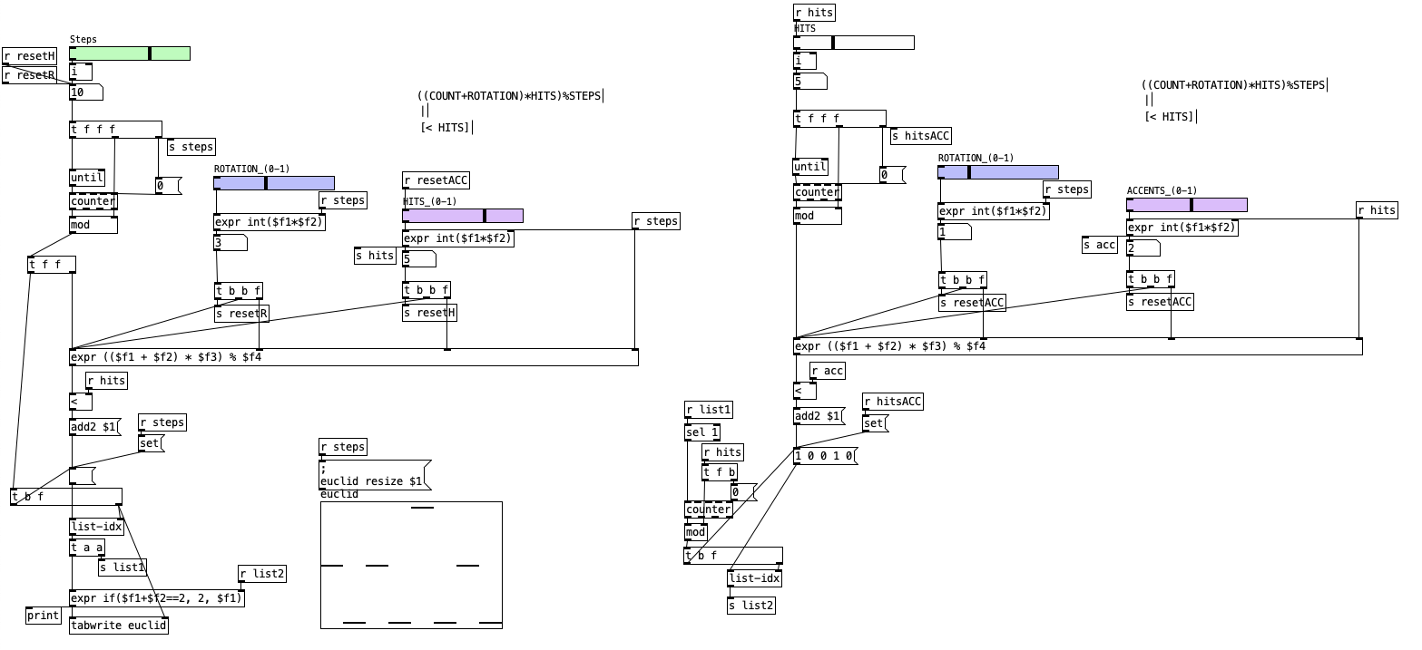
Euclidean accents generator showing two parallel Euclidean rhythm generators combined to create accented beat patterns with independent control over main rhythm and accent placement.

2.6.8.1 Patch Overview

The patch is organized into two parallel sections. The first section generates the main Euclidean rhythm, while the second section generates an accent pattern using the same mathematical approach. Both sections allow for independent control of steps, hits, rotation, and accents. The outputs of both patterns are then combined to produce a final sequence where steps can be silent, regular, or accented.

The following diagram illustrates the data flow for both rhythm and accent layers:

2.6.8.2 Data Flow

flowchart TD
    S[Steps Slider] --> A[Step Counter]
    H[Hits Slider] --> B[Hits Value]
    R[Rotation Slider] --> C[Rotation Value]
    A --> D[Euclidean Formula: index+rotation*hits%steps]
    B --> D
    C --> D
    D --> E[Compare < hits]
    E --> F[Main Pattern List]
    ACC[Accents Slider] --> ACCV[Accents Value]
    ACCROT[Accents Rotation Slider] --> ACCROTVAL[Accents Rotation Value]
    A2[Step Counter] --> D2[Euclidean Formula: index+acc_rotation*accents %steps]
    ACCV --> D2
    ACCROTVAL --> D2
    D2 --> E2[Compare < accents]
    E2 --> F2[Accent Pattern List]
    F & F2 --> G[Combine Patterns]
    G --> H[Output/Display]

The process begins with the user setting the number of steps, hits, and rotation for the main rhythm using horizontal sliders. These parameters determine the length of the sequence, the number of pulses, and the rotation (offset) of the pattern. The patch uses a loop (until) and a counter to iterate through each step index. For each step, it calculates the value using the formula ((index + rotation) * hits) % steps. This value is compared to the number of hits; if it is less, a pulse (1) is added to the main pattern, otherwise a rest (0).

In parallel, the user can set the number of accents and their rotation using additional sliders. The accent pattern is generated in the same way as the main rhythm, but with its own independent parameters. The formula ((index + acc_rotation) * accents) % steps is used to determine the placement of accents. The result is a second pattern of 1s (accent) and 0s (no accent).

After both patterns are generated, they are combined step by step. If both the main pattern and the accent pattern have a 1 at the same step, the output for that step is set to 2 (indicating an accented hit). If only the main pattern has a 1, the output is 1 (regular hit). If neither has a 1, the output is 0 (rest). The final combined pattern is written to an array and displayed, allowing for visualization and further use in sequencing.

2.6.8.3 Example: Combining Rhythm and Accents

Suppose you set 8 steps, 3 hits, and 2 accents. The main rhythm might produce a pattern like:

\[1 0 0 1 0 0 1 0\]

The accent pattern, with its own rotation, might produce:

\[1 0 1 0 0 1 0 0\]

Combining these, the output would be:

\[2 0 1 1 0 1 1 0\]

Here, “2” indicates an accented hit, “1” a regular hit, and “0” a rest.

2.6.8.4 Key Objects and Their Roles

Object	Purpose
`until`	Loops through each step index
`counter`	Increments the step index for each iteration
`expr`	Calculates the Euclidean formula for both rhythm and accent patterns
`<`	Compares the formula result to hits or accents, outputs 1 or 0
`add2`	Appends each result to the output pattern list
`list-idx`	Retrieves values from the generated lists for combination
`expr if($f1+$f2==2, 2, $f1)`	Combines main and accent patterns into a single output
`tabwrite`	Writes the final pattern to an array for visualization

2.7 Cellular Automata

Cellular automata are simple machines consisting of cells that update in parallel at discrete time steps. In general, the state of a cell depends on the state of its local neighborhood at the previous time step. The earliest known examples were engineered for specific purposes, such as the two-dimensional cellular automaton constructed by von Neumann in 1951 to model biological self-replication (Brummitt and Rowland 2012)

A cellular automaton is a mathematical and computational model for a dynamic system that evolves in discrete steps. It is suitable for modeling natural systems that can be described as a massive collection of simple objects interacting locally with each other.

A cellular automaton is a collection of “colored” cells on a grid of specified shape that evolves through a series of discrete time steps according to a set of rules based on the states of neighboring cells. The rules are then applied iteratively over as many time steps as desired.

Cellular automata come in a variety of forms and types. One of the most fundamental properties of a cellular automaton is the type of grid on which it is computed. The simplest such grid is a one-dimensional line. In two dimensions, square, triangular, and hexagonal grids can be considered.

One must also specify the number of colors (or distinct states) k that a cellular automaton can assume. This number is typically an integer, with k=2 (binary, [1] or [0]) being the simplest choice. For a binary automaton, color 0 is commonly referred to as “white” and color 1 as “black”. However, cellular automata with a continuous range of possible values can also be considered.

In addition to the grid on which a cellular automaton resides and the colors its cells can assume, one must also specify the neighborhood over which the cells influence each other.

2.7.1 One-Dimensional Cellular Automata (1DCA)

The simplest option is "nearest neighbors", where only the cells directly adjacent to a given cell can influence it at each time step. Two common neighborhoods in the case of a two-dimensional cellular automaton on a square grid are the so-called Moore neighborhood (a square neighborhood) and the von Neumann neighborhood (a diamond-shaped neighborhood).

Cellular automata are considered as a vector. Each component of the vector is called a cell. Each cell is assumed to take only two states:

[0] –> white

[1] –> black

This type of automaton is known as an elementary one-dimensional cellular automaton (1DCA). A dynamic process is performed, starting from an initial configuration C(0) of each of the cells (stage 0), and at each new stage, the state of each cell is calculated based on the state of the neighboring cells and the cell itself in the previous stage.

The cellular automata that we study in this section are one-dimensional. A one-dimensional cellular automaton consists of:

an alphabet Σ of size k,
a positive integer d,
a function i from the set of integers to Σ, and
a function f from Σ^d (d-tuples of elements in Σ) to S.

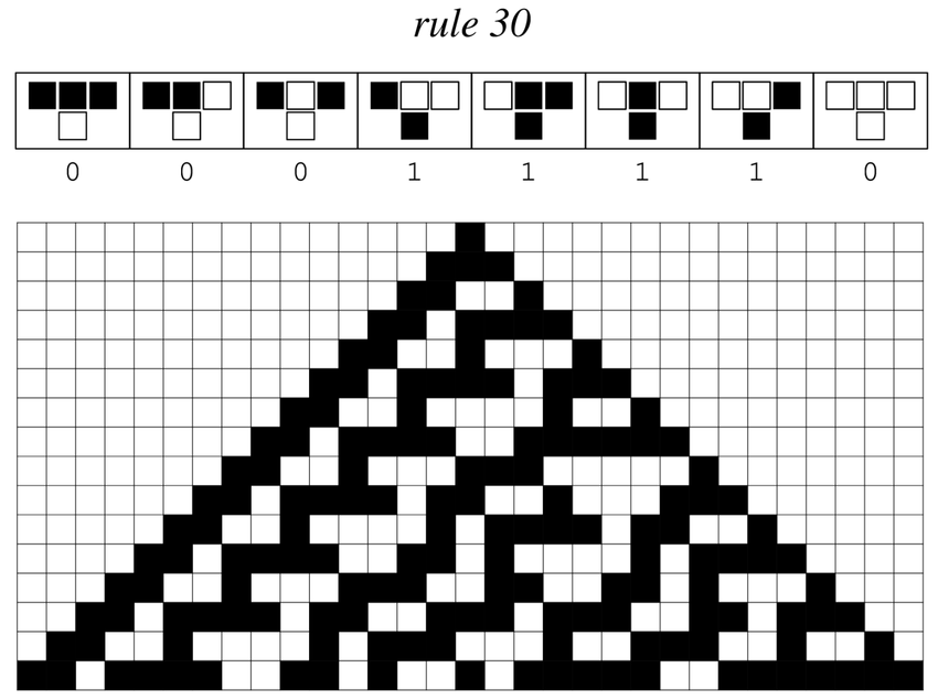
The function i is called the initial condition, and the function f is called the rule. We think of the initial condition as an infinite row of discrete cells, each assigned one of k colors. To evolve the cellular automaton, we update all cells in parallel, where each cell updates according to f, a function of d cells in its vicinity on the previous step. I adopt the usual convention of naming a cellular automaton’s rule by the number whose base-k digits consist of the outputs of the rule under the kd possible inputs of d cells, ordered reverse-lexicographically. For example, the two-color rule depending on three cells that maps the eight possible inputs according to the rule 00011110 = 30 in this numbering. Here we have identified 0 = [ ] and 1 = [x].

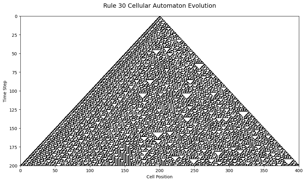
2.7.2 The Case of Rule 30

Rule 30 is a binary one-dimensional cellular automaton introduced by Stephen Wolfram (Wolfram 1983). It considers an infinite one-dimensional array of cellular automaton cells with only two states, with each cell in some initial state.

At discrete time intervals, each cell changes state spontaneously based on its current state and the state of its two neighbors.

What it consists of:

Each cell can be in one of two states: alive or dead.
The next generation of a cell is determined by the current state of the cell and the state of its two neighboring cells.
There are 8 possible configurations of neighboring states (3^2), and for each, Rule 30 defines whether the cell lives or dies in the next generation.

It is called Rule 30 because in binary, 00011110₂ = 30

For Rule 30, the set of rules that governs the automaton’s next state is:

Pattern (decimal)	Pattern (binary)	Next State (center cell)	New state (center cell)
0	000	Dead	000
1	001	Alive	011
2	010	Dead	000
3	011	Alive	011
4	100	Alive	011
5	101	Dead	000
6	110	Alive	011
7	111	Dead	000

In the following diagram, the top row shows the state of the central cell (cell i) and its two neighboring cells at a given stage, and the bottom row shows the state of the central cell in the next stage.

For example, in the first case of the figure:

if the state of a cell at a given stage is [1] (black) and
its two neighbors at that stage are also [1] (black),
then the cell’s state in the next stage will be [0] (white).

Rule 30 cellular automaton evolution displaying binary state transitions and emergent pattern generation from simple neighborhood-based rules.

Let’s break down the procedure for determining the next state in the 8 combinations:

Input configurations: Consider the 8 possible input combinations of the three cells (a central cell and its left and right neighbors). Since each cell can be in one of two possible states (0 or 1), the combinations are 000, 001, 010, 011, 100, 101, 110, and 111.

Binary representation of the rule: Rule 30 is represented by the number 30 in binary, which is 00011110. This binary representation determines the rules for the next state of the central cell for each of the 8 possible combinations.

Bit correspondence: The 8 bits of the binary representation (00011110) correspond to the 8 input combinations in order. From right to left, the bits represent the next state of the central cell for each input combination.

For example, the least significant bit of 00011110 (the rightmost bit) is 0. This means that when the input combination is 000, the next state of the central cell will be 0.

Next state determination: For each input combination (e.g., 000, 001, 010, 011, 100, 101, 110, 111), the corresponding bit in the binary representation of Rule 30 [00011110] indicates the next state of the central cell.

Input Configuration	Next State
000	0
001	1
010	1
011	1
100	1
101	0
110	0
111	0

For example, if the input combination is 000 and the corresponding bit in Rule 30 is 0, then the next state of the central cell will be 0.

Therefore, the rules are not arbitrary but are determined by the binary representation of Rule 30, which specifies the next state of the central cell for each input combination of its neighbors.

Rule 30 transition table illustrating the eight neighborhood patterns and their resulting center cell states for the next generation.

2.7.3 One-Dimensional Cellular Automata Implementation

his implementation demonstrates how to construct a one-dimensional cellular automaton system that can generate intricate sequences based on elementary rule sets. The patch showcases advanced concepts including rule-based pattern generation, boundary condition handling, state evolution tracking, and data persistence mechanisms.

One-dimensional cellular automaton patch implementing Rule 30 with iteration history display showing the evolution from a single seed cell into complex binary patterns.

Iteration	Binary Output
0	0 0 0 0 0 0 1 0 0 0 0 0
1	0 0 0 0 0 1 1 1 0 0 0 0
2	0 0 0 0 1 1 0 0 1 0 0 0
3	0 0 0 1 1 0 1 1 1 1 0 0
4	0 0 1 1 0 0 1 0 0 0 1 0
5	0 1 1 0 1 1 1 1 0 1 1 1
6	0 1 0 0 1 0 0 0 0 1 0 0
7	1 1 1 1 1 1 0 0 1 1 1 0
8	1 0 0 0 0 0 1 1 1 0 0 0
9	1 1 0 0 0 1 1 0 0 1 0 1
10	0 0 1 0 1 1 0 1 1 1 0 1
11	1 1 1 0 1 0 0 1 0 0 0 1
12	0 0 0 0 1 1 1 1 1 0 1 1
13	1 0 0 1 1 0 0 0 0 0 1 0
14	1 1 1 1 0 1 0 0 0 1 1 0
15	1 0 0 0 0 1 1 0 1 1 0 0
16	1 1 0 0 1 1 0 0 1 0 1 1
17	0 0 1 1 1 0 1 1 1 0 1 0
18	0 1 1 0 0 0 1 0 0 0 1 1
19	0 1 0 1 0 1 1 1 0 1 1 0
20	1 1 0 1 0 1 0 0 0 1 0 1
21	0 0 0 1 0 1 1 0 1 1 0 1
22	1 0 1 1 0 1 0 0 1 0 0 1
23	0 0 1 0 0 1 1 1 1 1 1 1

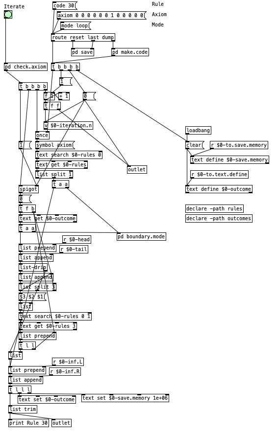
2.7.3.1 Patch Overview

The one-dimensional cellular automaton patch implements a comprehensive system for simulating elementary cellular automata, particularly focusing on Stephen Wolfram’s classification of 256 possible rules. The system operates by maintaining a linear array of cells, each containing a binary state (0 or 1), and applying transformation rules based on local neighborhoods of three consecutive cells. The patch provides sophisticated control over initial conditions (axioms), boundary behaviors, rule selection, and iteration management, making it suitable for both educational exploration and practical generative applications.

The architecture follows a modular design pattern with distinct functional subsystems that handle different aspects of the cellular automaton simulation. The rule management subsystem converts numerical rule codes into binary lookup tables that define state transitions for all possible three-cell neighborhoods. The boundary condition handler manages edge cases when the automaton reaches the limits of its defined space, supporting both loop-around and reflection modes. The iteration engine coordinates the step-by-step evolution of the cellular array, maintaining state history and providing real-time feedback on the generation process.

The patch interface accommodates various input methods for configuring the automaton parameters, including direct rule code entry (0-255), symbolic mode specification (loop, reflect, or fixed), and custom axiom definition through list messages. The system provides multiple output streams for accessing generated data, including real-time state information, complete iteration histories, and formatted data suitable for external analysis or visualization tools.

2.7.3.2 Data Flow

flowchart TD
    A[Rule Code Input] --> B[Binary Rule Generation]
    C[Axiom Definition] --> D[Initial State Setup]
    E[Mode Selection] --> F[Boundary Configuration]
    B --> G[Rule Lookup Table]
    D --> H[Current State Array]
    F --> I[Edge Handler]
    J[Iterate Bang] --> K[State Evolution Engine]
    H --> K
    G --> K
    I --> K
    K --> L[Next Generation]
    L --> M[State History]
    L --> N[Data Output]
    L --> H

The cellular automaton’s operation begins with initialization phase where the rule code, boundary mode, and initial axiom are processed and stored in the system’s internal data structures. The rule code undergoes binary conversion through a specialized subpatch that transforms decimal values (0-255) into their eight-bit binary representations, which correspond to the output states for all possible three-cell neighborhood configurations (000, 001, 010, 011, 100, 101, 110, 111).

The axiom processing system accepts list-formatted initial conditions that define the starting configuration of the cellular array. This initial state is stored in a text object that serves as both the current generation reference and the foundation for subsequent iterations. The boundary mode configuration determines how the system handles edge conditions when calculating neighborhoods for cells at the array boundaries, with options for periodic (loop), reflective, or fixed boundary conditions.

When an iteration is triggered through the iterate bang, the system enters its core evolution cycle. The current state array is processed through a neighborhood analysis routine that examines each cell in conjunction with its immediate neighbors. For each three-cell neighborhood, the system constructs a lookup key by treating the binary states as a three-bit number, which is then used to index into the previously generated rule table to determine the next state for the center cell.

The boundary condition handler plays a crucial role during this process, providing appropriate neighbor values for cells at the array edges based on the selected boundary mode. In loop mode, the array is treated as circular, with the leftmost and rightmost cells considered adjacent. Reflect mode mirrors the edge values inward, while fixed mode uses predetermined constant values for out-of-bounds references.

The resulting next generation is simultaneously output for immediate access and stored in the iteration history system. This dual-path approach allows for real-time monitoring of the automaton’s evolution while maintaining a complete record of all generated states. The history management system can accommodate both memory-efficient storage (retaining only the current state) and comprehensive archival (preserving all iterations) depending on the intended application.

2.7.3.3 Key Objects and Their Roles

The following table summarizes the essential objects and subsystems used in the cellular automaton implementation:

Object/Subsystem	Purpose
`make.code` subpatch	Converts rule codes to binary lookup tables and manages initialization
`float.to.binary` subpatch	Transforms decimal rule codes into 8-bit binary representations
`text define $0-rules`	Stores rule lookup table and configuration parameters
`text define $0-outcome`	Maintains current generation state and iteration history
`list-drip`	Processes cell arrays sequentially for neighborhood analysis
`list split 3`	Extracts three-cell neighborhoods from the current state
`text search`	Performs rule lookups based on neighborhood patterns
`text get`	Retrieves rule outcomes and state information
`boundary.mode` subpatch	Handles edge conditions and neighbor calculation
`list append/prepend`	Manages array concatenation and state assembly
`route`	Directs messages to appropriate processing subsystems
`v $0-iteration.n`	Tracks current iteration number and generation count
`save` subpatch	Provides data export functionality for generated sequences

The patch demonstrates several advanced programming techniques, including dynamic text object manipulation for rule storage, sophisticated list processing for array operations, and modular subpatch design for complex algorithmic implementations. The use of local variables ($0- prefix) ensures proper encapsulation when multiple instances of the patch are used simultaneously, while the declare objects manage external file dependencies for rule and outcome storage.

The cellular automaton implementation showcases how it can be used to create sophisticated algorithmic systems that bridge computational theory and practical creative applications. The modular architecture allows for easy experimentation with different rule sets, boundary conditions, and initial configurations, making it an excellent tool for exploring the rich behavioral space of elementary cellular automata and their potential applications in generative music, visual art, and algorithmic composition.

2.7.4 Two-Dimensional Cellular Automata (2DCA)

Two-dimensional cellular automata are an extension of one-dimensional cellular automata, where cells not only have neighbors to the left and right, but also above and below. This allows modeling of more complex and structurally rich systems, such as two-dimensional phenomena like wave propagation, growth patterns in biology, fire spread, fluid simulation, among others.

Two-dimensional cellular automata (2DCA) are computational models that simulate dynamic systems on a two-dimensional grid.

They consist of:

Cells: Each cell in the grid can have a finite state, such as alive or dead, and can change state according to the automaton’s rules.
Neighborhood: Each cell has a neighborhood, which is a set of adjacent cells that influence its state. The neighborhood can be rectangular, hexagonal, circular, or of any other shape.
Transition rule: The transition rule defines how the state of a cell changes based on its current state and the state of the cells in its neighborhood. The rule can be deterministic or probabilistic.
Evolution: The cellular automaton evolves through iterations. In each iteration, the state of each cell is updated according to the transition rule.

2.7.5 Case Study: Conway’s Game of Life

The most well known cellular automaton is the Game of Life, a two-dimensional cellular automaton which has been invented by John Horton Conway in 1970. It is a simulation that describes the evolution of a population of cells across a two-dimensional grid of squares by three (or four, depending on the wording) simple rules. Every cell has one of the two states ”dead” and ”alive”, and the state changes of the cells depend on the number of living neighbor cells. When it was first published by Martin Gardner in the journal Scientific American in 1970, it was praised to have ”fantastic combinations” (Gardner 1970). Since its invention, thousands of patterns have been found by many people, and there seems to be no end in sight. Even after more than 50 years of history, interesting new patterns are still discovered.

The “game” is actually a zero-player game, meaning its evolution is determined by its initial state, requiring no further input from human players. One interacts with the Game of Life by creating an initial configuration and observing how it evolves.

View Original Article - MATHEMATICAL GAMES - The fantastic combinations of John Conway’s new solitaire game life (Martin Gardner)

GOL (Game of Life) and CGOL (Conway’s Game of Life) are commonly used acronyms.

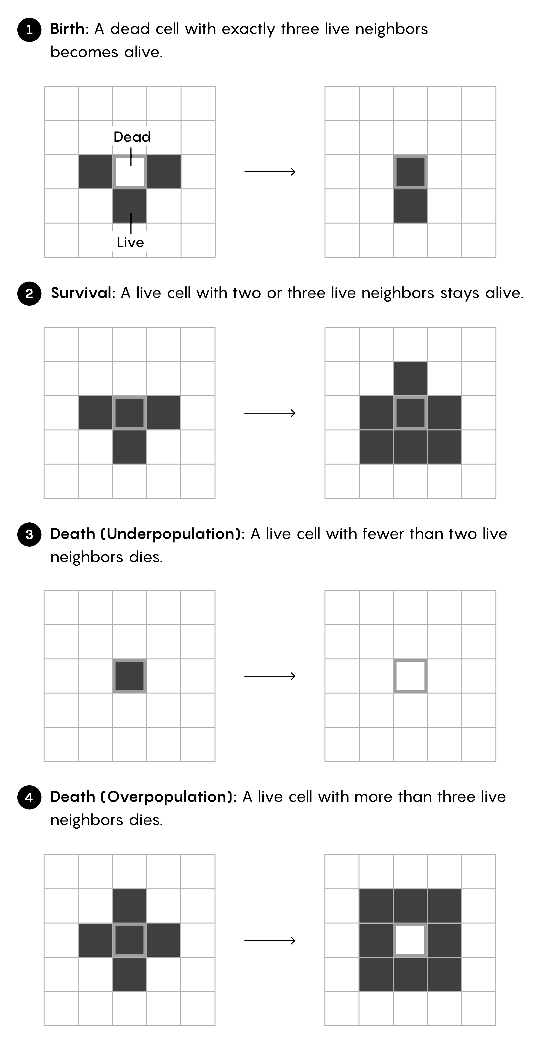
2.7.5.1 Rules

The universe of the Game of Life is an infinite two-dimensional orthogonal grid of square cells, each of which (at any given time) is in one of two possible states, alive (alternatively “on”) or dead (alternatively “off”). At each time step, the following transitions occur:

The four rules of Conway’s Game of Life:

1. Overpopulation: Any live cell with more than three live neighbors dies due to overpopulation.

2. Underpopulation: Any live cell with fewer than two live neighbors dies due to underpopulation.

3. Stability: Any live cell with two or three live neighbors survives to the next generation.

4. Reproduction: Any dead cell with exactly three live neighbors becomes a live cell.

We can also summarize the rules in a table:

Rule	Description	Current State	Live Neighbors	Next State
Overpopulation	Death by overcrowding	Alive	More than 3	Dead
Underpopulation	Death by isolation	Alive	Fewer than 2	Dead
Stability	Survival	Alive	2 or 3	Alive
Reproduction	Birth	Dead	3	Alive

Or summarized as

0 → 3 live neighbors → 1

1 → < 2 or > 3 live neighbors → 0

Where 0 represents a dead cell and 1 a live cell.

Game of Life rules diagram illustrating cell state transitions based on the number of living neighbors in the Moore neighborhood.

John Conway’s Game of Life is made of an infinite grid of square cells, each of which is alive or dead. The rules below govern the evolution of the system. Every cell has eight neighbors, and all cells update simultaneously as time advances.

Conway’s Game of Life rule visualization showing the four fundamental rules governing cell evolution: underpopulation, survival, reproduction, and overpopulation based on neighbor count.

The initial pattern constitutes the system’s ‘seed’. The first generation is created by applying the above rules simultaneously to each cell in the seed; births and deaths occur simultaneously, and the discrete moment in which this occurs is sometimes called a step. (In other words, each generation is a pure function of the previous one.) The rules continue to be applied repeatedly to create more generations.

2.7.6 Origins

Conway was interested in a problem presented in the 1940s by renowned mathematician John von Neumann, who was trying to find a hypothetical machine that could build copies of itself and succeeded when he found a mathematical model for such a machine with very complicated rules on a rectangular grid. The Game of Life emerged as Conway’s successful attempt to simplify von Neumann’s ideas.

The game made its first public appearance in the October 1970 issue of Scientific American, in Martin Gardner’s “Mathematical Games” column, under the title “The fantastic combinations of John Conway’s new solitaire game ‘Life’”.

Since its publication, Conway’s Game of Life has attracted significant interest due to the surprising ways patterns can evolve.

Life is an example of emergence and self-organization. It is of interest to physicists, biologists, economists, mathematicians, philosophers, generative scientists, and others, as it shows how complex patterns can emerge from the implementation of very simple rules. The game can also serve as a didactic analogy, used to convey the somewhat counterintuitive notion that “design” and “organization” can spontaneously arise in the absence of a designer.

Conway carefully selected the rules, after considerable experimentation, to meet three criteria:

There should be no initial pattern for which a simple proof exists that the population can grow without limit.
There must be initial patterns that appear to grow indefinitely.
There should be simple initial patterns that evolve and change for a considerable period before ending in one of the following ways:
- dying out completely (due to overcrowding or becoming too sparse); or
- settling into a stable configuration that remains unchanged thereafter, or entering an oscillating phase in which they repeat a cycle endlessly of two or more periods.

2.7.7 Patterns

Many different types of patterns occur in the Game of Life, including static patterns (“still lifes”), repeating patterns (“oscillators” – a superset of still lifes), and patterns that move across the board (“spaceships”). Common examples of these three classes are shown below, with live cells in black and dead cells in white.

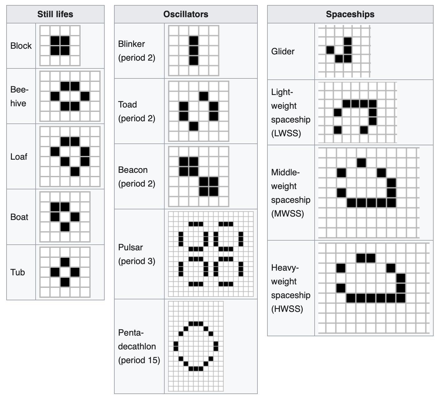
Using the provided rules, you can investigate the evolution of simple patterns:

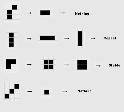
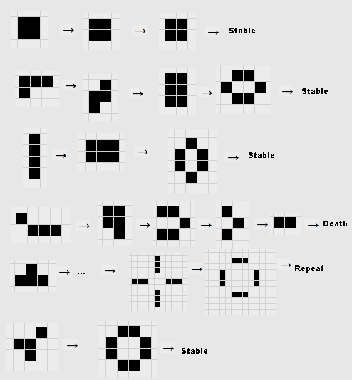
Patterns that evolve for long periods before stabilizing are called Methuselahs, the first of which discovered was the R-pentomino.

Diehard is a pattern that eventually disappears, rather than stabilizing, after 130 generations, which is believed to be the maximum for initial patterns with seven or fewer cells.

Acorn takes 5,206 generations to produce 633 cells, including 13 escaping gliders.

Conway originally conjectured that no pattern could grow indefinitely; that is, for any initial configuration with a finite number of live cells, the population could not grow beyond some finite upper bound. The Gosper glider gun pattern produces its first glider in the 15th generation, and another every 30 generations thereafter.

For many years, this pattern was the smallest known. In 2015, a gun called Simkin glider gun was discovered, which emits a glider every 120 generations, and has fewer live cells but is spread across a larger bounding box at its ends.

For a more detailed overview of gliders and other patterns, you can refer and extensive post by Swaraj Kalbande Conway’s Game of Life-Life on Computer (Kalbande 2022).

2.7.8 Python Implementation of Game of Life

import time
import pygame
import numpy as np

COLOR_BG = (10, 10, 10,)  # Color de fondo
COLOR_GRID = (40, 40, 40)  # Color de la cuadrícula
COLOR_DIE_NEXT = (170, 170, 170)  # Color de las células que mueren en la siguiente generación
COLOR_ALIVE_NEXT = (255, 255, 255)  # Color de las células que siguen vivas en la siguiente generación

pygame.init()
pygame.display.set_caption("conway's game of life")  # Título de la ventana del juego

# Función para actualizar la pantalla con las células
def update(screen, cells, size, with_progress=False):
    updated_cells = np.zeros((cells.shape[0], cells.shape[1]))  # Matriz para almacenar las células actualizadas

    for row, col in np.ndindex(cells.shape):
        alive = np.sum(cells[row-1:row+2, col-1:col+2]) - cells[row, col]  # Cálculo de células vecinas vivas
        color = COLOR_BG if cells[row, col] == 0 else COLOR_ALIVE_NEXT  # Color de la célula actual

        if cells[row, col] == 1:  # Si la célula actual está viva
            if alive < 2 or alive > 3:  # Si tiene menos de 2 o más de 3 vecinos vivos, muere
                if with_progress:
                    color = COLOR_DIE_NEXT
            elif 2 <= alive <= 3:  # Si tiene 2 o 3 vecinos vivos, sigue viva
                updated_cells[row, col] = 1
                if with_progress:
                    color = COLOR_ALIVE_NEXT
        else:  # Si la célula actual está muerta
            if alive == 3:  # Si tiene exactamente 3 vecinos vivos, revive
                updated_cells[row, col] = 1
                if with_progress:
                    color = COLOR_ALIVE_NEXT

        pygame.draw.rect(screen, color, (col * size, row * size, size - 1, size - 1))  # Dibuja la célula en la pantalla

    return updated_cells  # Devuelve las células actualizadas

# Función principal del programa
def main():
    pygame.init()
    screen = pygame.display.set_mode((800, 600))  # Crea la ventana del juego

    cells = np.zeros((60, 80))  # Crea una matriz de células muertas
    screen.fill(COLOR_GRID)  # Rellena la pantalla con el color de la cuadrícula
    update(screen, cells, 10)  # Actualiza la pantalla con las células

    pygame.display.flip()
    pygame.display.update()

    running = False  # Variable para controlar si el juego está en ejecución

    while True:
        for Q in pygame.event.get():
            if Q.type == pygame.QUIT:  # Si se cierra la ventana, termina el programa
                pygame.quit()
                return
            elif Q.type == pygame.KEYDOWN:
                if Q.key == pygame.K_SPACE:  # Si se presiona la tecla espacio, se inicia o pausa el juego
                    running = not running
                    update(screen, cells, 10)
                    pygame.display.update()
            if pygame.mouse.get_pressed()[0]:  # Si se presiona el botón izquierdo del ratón
                pos = pygame.mouse.get_pos()  # Obtiene la posición del ratón
                cells[pos[1] // 10, pos[0] // 10] = 1  # Marca la célula correspondiente como viva
                update(screen, cells, 10)
                pygame.display.update()

        screen.fill(COLOR_GRID)  # Rellena la pantalla con el color de la cuadrícula

        if running:  # Si el juego está en ejecución
            cells = update(screen, cells, 10, with_progress=True)  # Actualiza las células con progreso
            pygame.display.update()

        time.sleep(0.001)  # Espera un breve tiempo para controlar la velocidad del juego

if __name__ == "__main__":
    main()

This Python script implements Conway’s Game of Life, a cellular automaton devised by British mathematician John Horton Conway. It is a zero-player game, meaning its evolution is determined entirely by its initial state, with no further input required.

The script begins by importing the necessary modules: time, pygame for the graphical interface, and numpy to handle the game grid as a 2D matrix. It then defines color constants used for visualizing the game.

The pygame.init() function is called to initialize all imported Pygame modules. The window title is set to “Conway’s Game of Life” using pygame.display.set_caption().

The update() function updates the game state and redraws the grid. It takes four arguments: screen (the Pygame surface to draw on), cells (the current game state as a 2D numpy array), size (the pixel size of each cell), and with_progress (a boolean indicating whether to display cells that will change in the next generation).

The function creates a new 2D matrix updated_cells filled with zeros, matching the shape of cells. It then iterates over each cell, calculates the number of live neighbors, and applies the game rules to determine whether the cell will be alive in the next generation. The function draws each cell on the screen using the appropriate color and returns updated_cells.

The main() function initializes Pygame, creates the game window, and initializes the game state as a 2D numpy array of zeros (representing dead cells). It then enters the main loop, which handles Pygame events (such as closing the window or key presses), updates the game state if it is running, and redraws the grid. The game can be started or paused by pressing the spacebar, and cells can be toggled manually by clicking on them.

Finally, the script calls main() to launch the game. Press the spacebar to begin.

2.7.9 Further Reading

2.7.10 Interactive Websites

References

Brown, Andrew. 2023. “Live Coding Patterns and a Toolkit for Pure Data.” Organised Sound 28: 1–12. https://doi.org/10.1017/S1355771823000365.

Brummitt, Charles D., and Eric Rowland. 2012. “Boundary Growth in One-Dimensional Cellular Automata.” Complex Systems 21: 85–116. https://doi.org/10.48550/arXiv.1204.2172.

Epstein, Paul. 1986. “Pattern Structure and Process in Steve Reich’s Piano Phase.” The Musical Quarterly 72 (4): 494–502.

Gardner, Martin. 1970. “MATHEMATICAL GAMES - the Fantastic Combinations of John Conway’s New Solitaire Game Life.” Scientific American 223 (4): 120–23. http://www.jstor.org/stable/24927642.

Kalbande, Swaraj. 2022. “Conway’s Game of Life – Life on Computer.” Medium. https://medium.com/@swarajkalbande123/conways-game-of-life-life-on-computer-b7edfc85d21a.

Reich, Steve. 2002. “Music as a Gradual Process.” In Writings on Music 1965–2000, 34–36. Oxford; New York: Oxford University Press.

Toussaint, Godfried. 2005. “The Euclidean Algorithm Generates Traditional Musical Rhythms.” In, 47–56.

Wolfram, Stephen. 1983. “Statistical Mechanics of Cellular Automata.” Reviews of Modern Physics 55 (3): 601–44. https://doi.org/10.1103/RevModPhys.55.601.